Multiple Object Tracking
Posted on (Update: )
This note is for Luo, W., Xing, J., Milan, A., Zhang, X., Liu, W., Zhao, X., & Kim, T.-K. (2014). Multiple Object Tracking: A Literature Review. ArXiv:1409.7618 [Cs].
Introduction
The task of MOT (Multiple Object Tracking), or MMT (Multiple Target Tracking), is largely partitioned to locating multiple objects, maintaining their identities, and yielding their individual trajectories given an input video.
As a mid-level task in computer vision, multiple object tracking grounds high-level tasks such as pose estimation, action recognition, and behavior analysis.
Compared with Single Object Tracking (SOT), which primarily focuses on designing sophisticated appearance models and/or motion models to deal with challenging factors such as scale changes, out-of-plane rotations and illumination variations, MOT additionally requires two tasks to be solved: determining the number of objects, which typically varies over time, and maintaining their identities.
Apart from the common challenges in both SOT and MOT, further key issues that complicate MOT include among others:
- frequent occlusions
- initialization and termination of tracks
- similar appearance
- interactions among multiple objects
Differences from Other Related Reviews
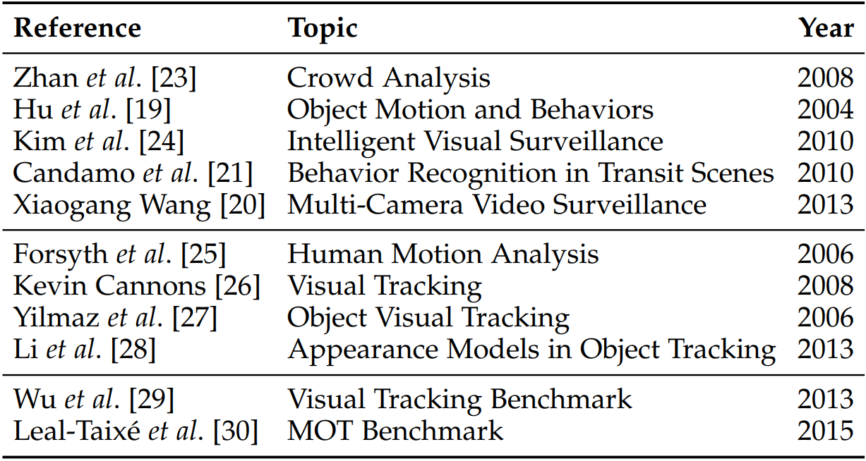
- the first set discusses tracking as an individual part while this work specifically discusses various aspects of MOT.
- the second set is dedicated to general visual tracking techniques or some special issues such as appearance models in visual tracking
- the third set introduces and discusses benchmarks on general visual tracking and on specific multiple object tracking, which focus on experimental studies rather than literature reviews.
MOT Problem
In general, multiple object tracking can be viewed as a multi-variable estimation problem. Given an image sequence, employ $\s_t^i$ to denote the state of the $i$-th object in the $t$-th frame, $\S_t=(\s_t^1,\ldots,\s_t^{M_t})$ to denote state of all the $M_t$ objects in the $t$-th frame. Let $\s_{i_s:i_e}^i=\{\s_{i_s}^i,\ldots,\s_{i_e}^i\}$ denote the sequential states of the $i$-th object, where $i_s$ and $i_e$ are respectively the first and last frame in which target $i$ exists, and $\S_{1:t}=\{\S_1,\ldots,\S_t\}$ denote all the sequential states of all the objects from the first frame to the $t$-th frame.
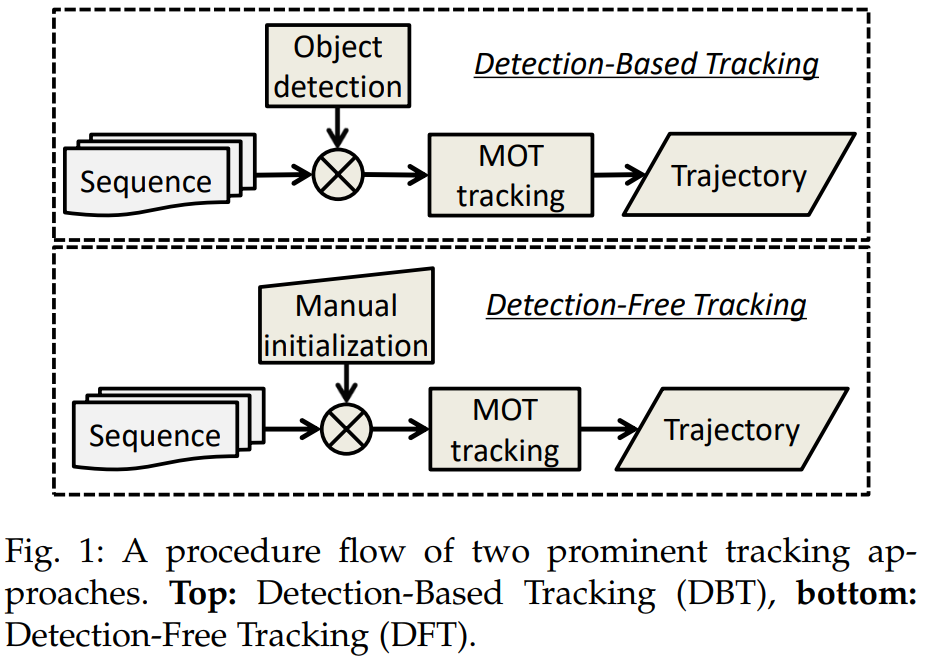
Following the most commonly used tracking-by-detection, or Detection Based Tracking (DBT) paradigm, utilize $\o_t^i$ to denote the collected observations for the $i$-th object in the $t$-th frame, $\O_t=(\o_1^1,\o^2_t,\ldots,\o^{M_t}_t)$ to denote all the collected sequential observations of all the objects from the first frame to the $t$-th frame.
The object of multiple object tracking is to find the “optimal” sequential states of all the objects, which can be generally modelled by performing MAP (maximal a posteriori) estimation from the conditional distribution of the sequential states given all the observations
\[\hat\S_{1:t} = \argmax_{\S_{1:t}}\; P(\S_{1:t}\mid \O_{1:t})\]Different MOT algorithms can be thought as designing different approaches to solving the above MAP problem, either from a probabilistic inference perspective or a deterministic optimization perspective.
The probabilistic inference based approaches usually solve the MAP problem using a two-step iterative procedures as follows:
- Predict: $P(\S_t\mid \O_{1:t-1})=\int P(\S_t\mid \S_{t-1})P(\S_{t-1}\mid \O_{1:t-1})d\S_{t-1}$
- Update: $P(\S_t\mid \O_{1:t})\propto P(\O_t\mid \S_t)P(\S_t\mid \O_{1:t-1})$.
Here $P(\S_t\mid \S_{t-1})$ and $P(\O_t\mid \S_t)$ are the Dynamic Model and the Observation Model, respectively.(Refer here for a detailed derivation.)
The deterministic optimization based approaches directly maximize the likelihood function $L(\O_{1:t}\mid \S_{1:t})$ as a delegate of $P(\S_{1:t}\mid \O_{1:t})$ over a set of available observations $\{\hat \O_{1:t}^n\}$:
\[\begin{align*} \hat \S_{1:t} &= \argmax_{\S_{1:t}}P(\S_{1:t}\mid \O_{1:t})\\ &= \argmax_{\S_{1:t}}L(\O_{1:t}\mid \S_{1:t})\\ &= \argmax_{\S_{1:t}}\prod_n P(\hat\O_{1:t}^n\mid \S_{1:t})\,, \end{align*}\](why $n$?) or conversely minimize an energy function $E(\S_{1:t}\mid \O_{1:t})$.
MOT Categorization
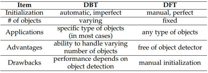
Initialization method
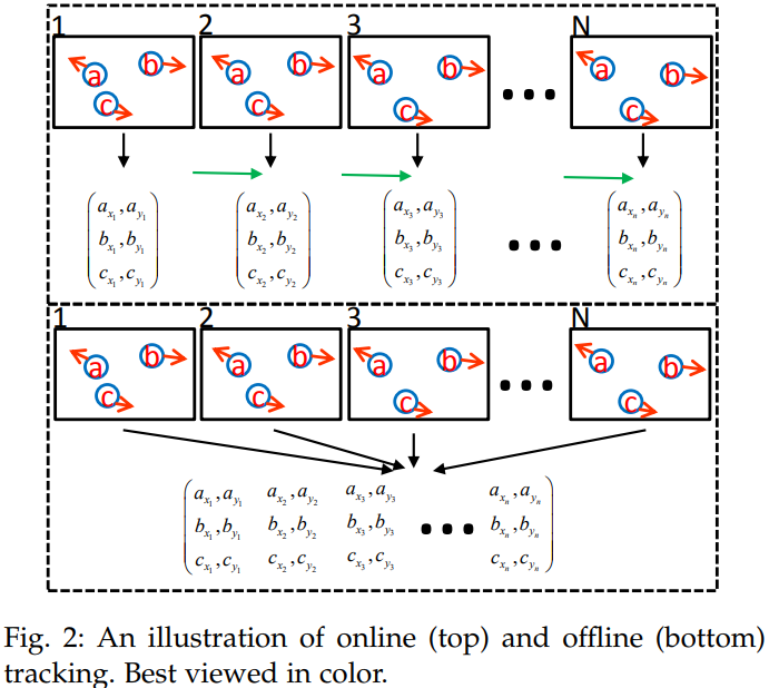
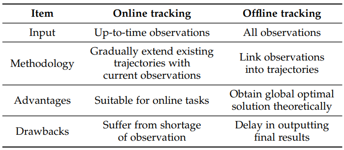
Processing Mode
Type of Output
probabilistic or deterministic
MOT Components
Two major issues:
- how to measure similarity between objects in frames
- how to recover the identity information based on the similarity measurement between objects across frames
Appearance Model
Appearance is an important cue for affinity computation in MOT. Technically, an appearance model includes two components:
- visual representation: describe the visual characteristics of an object using some features, either based on a single cue or multiple cues.
- statistical measuring: the computation of similarity between different observations.
Visual Representation
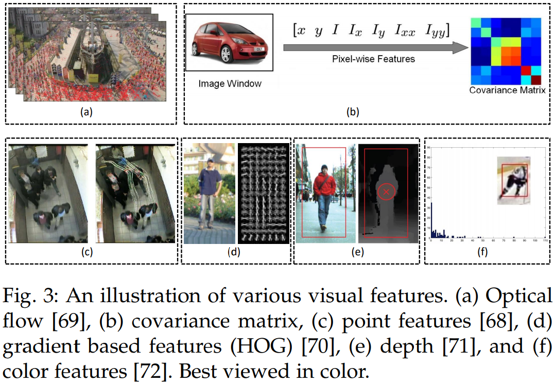
- Local features
- Region features
- zero-order: color histogram
- first-order: gradient-based representation
- up-to-second-order: region covariance matrix
- Others
Statistical Measuring
- Single cue: either transforming distance into similarity or directly calculating the affinity. For example, Bhattacharyya distance $B(\cdot,\cdot)$ is used to compute the distance between two color histograms $\c_i$ and $\c_j$. The distance is transformed into similarity $S$ like $S(\T_i,\T_j)=\exp(-B(\c_i,\c_j))$.
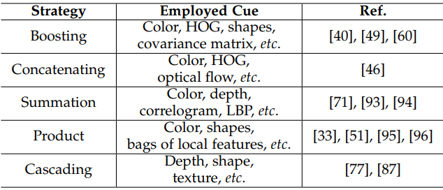
- Multiple cue: different kinds of cues can complement each other to make the appearance model more robust. But it is not trivial to decide how to fuse the information from multiple cues. Summarize multicue based appearance models according to five kinds of fusion strategies.
Motion Model
The motion model captures the dynamic behavior of an object. It estimates the potential position of objects in the future frames, thereby reducing the search space.
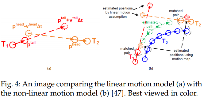
Linear Motion Model
- velocity smoothness is modeled by enforcing the velocity values of an object in successive frames to change smoothly. Someone implements it as a cost term,
where the summation is conducted over $N$ frames and $M$ trajectories/objects.
- position smoothness directly forces the discrepancy between the observed position and estimated position. For example, consider a temporal gap $\Delta t$ between tail of tracklet $T_j$ and head of tracklet $T_i$, the smoothness is modeled by fitting the estimated position to a Gaussian distribution with the observed position as center.
- acceleration smoothness
Non-linear Motion Model
Interaction Model
Social Force Models
Also known as group models. In these models, each object is considered to be dependent on other objects and environmental factors. This type of information could alleviate performance deterioration in crowded scenes. Specifically, in social force models, target behavior is modeled based on two aspects, individual force and group force.
- Individual force: fidelity and constancy
- Group force: attraction, repulsion, coherence
The majority of existing publications modeling interaction among objects with social force typically minimizes an energy objective, consisting of terms reflecting individual force and group force.
Crowd Motion Pattern Models
Motion patterns are introduced to alleviate the difficulty of tracking an individual object in the crowd. In general, this type of models is usually applied in the over-crowded scenario where the density of targets is considerably high.
Two kinds of motion patterns,
- structured: exhibit collective spatio-temporal structure
- unstructured: exhibit various modalities of motion
Exclusion Model
two constraints:
- detection-level exclusion
- trajectory-level exclusion
Detection-level Exclusion Modeling
- soft modeling: minimize a cost term to penalize the case of violation
- hard modeling: apply explicit constraint
Trajectory-level Exclusion Modeling
penalize the case that two close detection hypotheses have different trajectory labels
Occlusion Handling
perhaps the most critical challenge in MOT. A primary cause for ID switches or fragmentation of trajectories.
Part-to-whole
this strategy is built on the assumption that a part of the object is still visible when an occlusion happens.
the popular way is dividing a holistic object into several parts and computing affinity based on individual parts.
Hypothesize-and-test
generate occlusion hypotheses and then test it
Buffer-and-recover
buffers observations when occlusion happens and remembers states of objects before occlusion. When occlusion ends, object states are recovered based on the buffered observations and the stored states before occlusion.
Others
Inference
Probabilistic Inference
Approaches based on probabilistic inference typically represent states of objects as a distribution with uncertainty. The goal of a tracking algorithm is to estimate the probabilistic distribution of target state by a variety of probability reasoning methods based on existing observations.
This kind of approaches typically requires only the existing, past and present observations, thus they are especially appropriate for the task of online tracking. As only the existing observations are employed for estimation, it is naturally to impose the assumption of Markov property in the objects state sequence, which has two aspects:
- $P(\S_t\mid \S_{1:t-1})=P(\S_t\mid \S_{t-1})$
- $P(\O_{1:t}\mid \S_{1:t})=\prod_{i=1}^tP(\O_t\mid \S_t)$
models:
- Kalman filter
- Extended Kalman filter
- Particle filter
Deterministic Optimization
Approaches within this framework are more suitable for the task of offline tracking. Given observations (usually detection hypotheses) from all the frames, these types of methods endeavor to globally associate observations belonging to an identical object into a trajectory. The key issue is how to find the optimal association.
Popular and well-studies approaches:
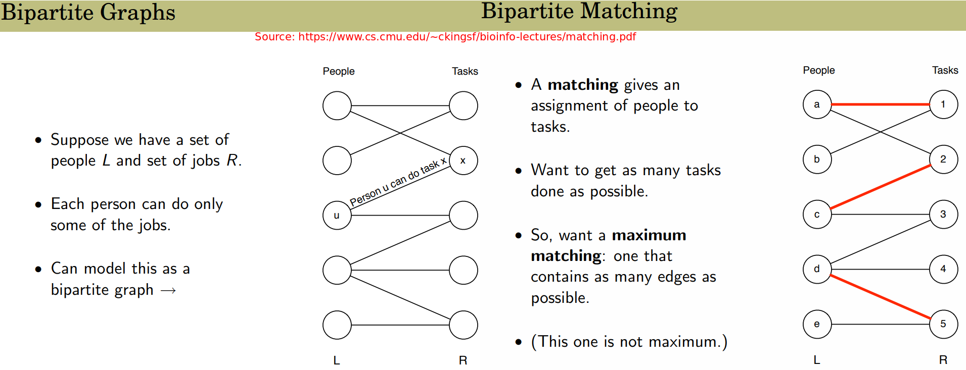
- Bipartite graph matching
- Dynamic Programming
- Min-cost max-flow network flow: nodes in the graph are detection responses or tracklets. Flow is modeled as an indicator to link two nodes or not. One trajectory corresponds to one flow path in the graph.
- Conditional random field.
- MWIS, maximum-weight independent set
Discussion
- probabilistic approaches provide a more intuitive and complete solution to the problem
- energy minimization could obtain a good enough solution in a reasonable time
Model Evaluation
Metrics
Metrics for Detection
- Accuracy
- Precision
Metrics for Tracking
- Accuracy
- Precision
- Completeness
- Robustness
Datasets
Public Algorithms
Benchmark Results
Summary
Existing Issues
- performance of an MOT method depends heavily on the object detectors
- many parameters need to be tuned.
Further Directions
- MOT with video adaptation
- MOT under multiple cameras
- Multiple 3D object tracking
- MOT with scene understanding
- MOT with deep learning
- MOT with other computer vision tasks