Particle Filtering and Smoothing

Posted on Jan 18, 2019 (Update: Apr 09, 2019) 0 Comments

This note is for Doucet, A., & Johansen, A. M. (2009). A tutorial on particle filtering and smoothing: Fifteen years later. Handbook of Nonlinear Filtering, 12(656–704), 3. For the sake of clarity, I split the general SMC methods (section 3) into my next post.

Abstract

1. Optimal estimation problems for non-linear non-Gaussian state-space models do not typically admit analytic solutions.
2. Particle filtering methods have become a very popular class of algorithms to solve these estimation problems numerically in an online manner, i.e., recursively as observations become available.

Introduction

1. The general state space hidden Markov models provide an extremely flexible framework for modelling time series.
2. It is impossible to obtain analytic solutions to the inference problems of interest with the exception of a small number of particularly simple cases.
3. The “particle” method are a broad and popular class of Monte Carlo algorithms which can provide approximate solutions to these intractable inference problems.
4. In comparison with standard approximation methods, such as the popular Extended Kalman Filter, the principal advantage of particle methods is that they do not rely on any local linearisation technique or any crude functional approximation.

Bayesian Inference in Hidden Markov Models

HMM and Inference Aims

Consider an $\cX$-valued discrete-time Markov process $\{X_n\}_{n\ge 1}$ such that

We are interested in estimating $\{X_n\}_{n\ge 1}$ but only have access to the $\cY$-valued process $\{Y_n\}_{n\ge 1}$. Assume that, given $\{X_n\}_{n\ge 1}$, the observations $\{Y_n\}_{n\ge 1}$ are statistically independent and their marginal densities are

Only consider the homogeneous case, which means that the transition and observation densities are independent of the time index $n$.

Model compatible with $\eqref{eq1}$-$\eqref{eq2}$ are known as hidden Markov models (HMM) or general state-space models (SSM).

Examples

1. Finite State-Space HMM.
2. Linear Gaussian model
3. Switching Linear Gaussian model
4. Stochastic Volatility model

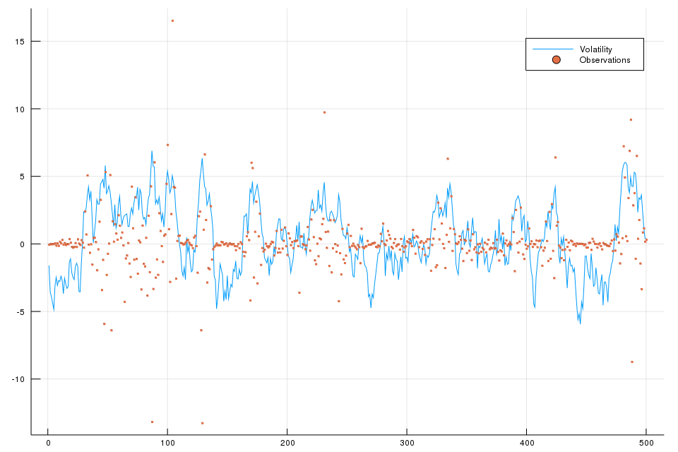
In particular, the stochastic volatility model can be written as

where $V_n\iid N(0,1)$ and $W_n\iid N(0,1)$. In this case, we have

We can use the following code to reproduce Figure 1 of the stochastic volatility model.

using Distributions
using Plots
using Random

Random.seed!(99);

α = 0.91
β = 0.5
σ = 1.0

T = 500
x = zeros(T)
Y = zeros(T)
x[1] = rand(Normal(0, σ/sqrt(1-α^2)))
Y[1] = rand(Normal(0, β*exp(x[1]/2)))
for t = 2:T
    x[t] = rand(Normal(α*x[t-1], σ))
    Y[t] = rand(Normal(0, β*exp(x[t]/2)))
end

plot(x, label="Volatility", size = (960, 640))
scatter!(Y, marker = (:none, 1), label = "Observations")
savefig("sv.png")

Equations $\eqref{eq1}$-$\eqref{eq2}$ define a Bayesian model:

and

In such a Bayesian context, inference about $X_{1:n}$ given a realisation of the observations $Y_{1:n}=y_{1:n}$ relies upon the posterior distribution

For most non-linear non-Gaussian models, it is not possible to compute these distributions in closed-form and we need to employ numeric methods. Particles methods are a set of flexible and powerful simulation-based methods which provide samples approximately distributed according to posterior distributions of the form $p(x_{1:n},y_{1:n})$ and facilitate the approximation calculation of $p(y_{1:n})$. Such methods are a subset of the class of methods known as Sequential Monte Carlo methods.

Two problems:

• Filtering and Marginal likelihood computation: Sequential approximation of the distributions $\{p(x_{1:n}\mid y_{1:n})\}_{n\ge 1}$ and marginal likelihoods $\{p(y_{1:n})\}_{n\ge 1}$. That is, approximate $p(x_1\mid y_1)$ and $p(y_1)$ at the first time instance, and so on. This problem is referred as optimal filtering problem.
• Smoothing: Sample from a joint distribution $p(x_{1:T}\mid y_{1:T})$ and approximate associated marginals $\{p(x_n\mid y_{1:T})\}$ where $n=1,\ldots,T$.

Filtering and Marginal Likelihood

The problem of filtering: characterising the distribution of the state of the hidden Markov model at the present time, given the information provided by all of the observations received up to the present time. This can be thought of as a “tracking” problem: keeping track of the current “location” of the system given noisy observations. This term is sometimes also used to refer to the practice of estimating the full trajectory of the state sequence up to the present time given the observations received up to this time.

“has been dedicated from the outset”: 从一开始就致力于

Note that

where

And we can get

where the $\color{blue}{\text{blue term}}$ is referred as the updating step, while the $\color{red}{\text{red term}}$ is known as the prediction step. However, most particle filtering methods rely on a numerical approximation of recursion $\eqref{eq9}$ and not of $\eqref{eq11}$.

If we can compute $\{p(x_{1:n}\mid y_{1:n})\}$ and thus $\{p(x_n\mid y_{1:n})\}$ sequentially, then the quantity $p(y_{1:n})$, which is known as the marginal likelihood, can also clearly be evaluated recursively using

where $p(y_k\mid y_{1:k-1})$ is of the form $\eqref{eq10}$.

Smoothing

Whereas filtering corresponds to estimating the distribution of the current state of an HMM based upon the observations received up until the current time, smoothing corresponds to estimating the distribution of the state at a particular time given all of the observations up to some later time. The trajectory estimates obtained by such methods, as a result of the additional information available, tend to be smoother than those obtained by filtering.

More formally: assume that we have access to the data $y_{1:T}$, and wish to compute the marginal distributions $\{p(x_n\mid y_{1:T})\}$ where $n=1,\ldots,T$ or to sample from $p(x_{1:T}\mid y_{1:T})$. In principle, the marginals $\{p(x_n\mid y_{1:T})\}$ could be obtained directly by considering the joint distribution $p(x_{1:T}\mid y_{1:T})$ and integrating out the variables $(x_{1:n-1},x_{n+1:T})$.

Forward-Backward Recursions

Decompose the joint distribution $p(x_{1:T}\mid y_{1:T})$ as follows:

$\{X_n\}$ is an inhomogeneous Markov process conditional on $y_{1:T}$.

To sample from $p(x_{1:T}\mid y_{1:T})$:

1. compute and store the marginal distributions $\{x_n\mid y_{1:n}\}$ for $n=1,\ldots,T$;
2. sample $X_T\sim p(x_T\mid y_{1:T})$
3. for $n=T-1,T-2,\ldots,1$, sample $X_n\sim p(x_n\mid X_{n+1},y_{1:n})$, where \(p(x_n\mid x_{n+1},y_{1:n})=\frac{f(x_{n+1}\mid x_n,y_{1:n})p(x_n\mid y_{1:n})}{p(x_{n+1}\mid y_{1:n})}=\frac{f(x_{n+1}\mid x_n)p(x_n\mid y_{1:n})}{p(x_{n+1}\mid y_{1:n})}\)

By integrating out $(x_{1:n-1},x_{n+1:T})$ in $\eqref{eq14}$,

Generalised Two-Filter Formula

Consider the following identity

where the so-called backward information filter is initialised at time $n=T$ by $p(y_T\mid x_T)=g(y_T\mid x_T)$ and satisfies

The backward information filter is not a probability density in argument $x_n$ and it is even possible that $\int p(y_{n:T}\mid x_n)dx_n=\infty$.

why integrate with respect to $x_n$??

A generalised version of the two-filter formula relies on the introduction of a set of artificial probability distributions $\{\tilde p_n(x_n)\}$ and the joint distributions

which are constructed such that their marginal distributions, $\tilde p_n(x_n\mid y_{n:T})\propto \tilde p_n(x_n)p(y_{n:T}\mid x_n)$ are simply “integrable versions” of the backward information filter. It is easy to establish the generalised two-filter formula

which is valid whenever the support of $\tilde p_n(x_n)$ includes the support of the prior $p_n(x_n)$; that is

The generalised two-filter smoother for $\{p(x_n\mid y_{n:T})\}$ proceeds as follows:

1. compute and store the marginal distributions $\{p(x_n\mid y_{1:n-1})\}$ via the standard forward recursion;
2. compute and store $\{\tilde p(x_n\mid y_{n:T})\}$ via a backward recursion;
3. for any $n=1,\ldots,T$, we can combine $p(x_n\mid y_{1:n-1})$ and $\tilde p(x_n\mid y_{n:T})$ to obtain $p(x_n\mid y_{1:T})$.

Particle Filtering

In the filtering context, we want to compute a numerical approximation of the distribution $\{p(x_{1:n}\mid y_{1:n})\}$ sequentially in time.

SMC for Filtering

Firstly, consider the simplest case in which $\gamma_n(x_{1:n})=p(x_{1:n},y_{1:n})$ is chosen, yielding $\pi_n(x_{1:n})=p(x_{1:n}\mid y_{1:n})$ and $Z_n=p(y_{1:n})$. It is only necessary to choose the importance distribution $q_n(x_n\mid x_{1:n-1})$. In order to minimise the variance of the importance weights at time $n$, we should select $q_n^{opt}(x_n\mid x_{1:n-1})=\pi_n(x_n\mid x_{1:n-1})$ where

and the associated incremental importance weight is $\alpha_n(x_{1:n})=p(y_n\mid x_{n-1})$.

Note that the target distribution is not $\pi_n(x_{1:n})$, but with some normalized constant, then the incremental importance weight would not be exactly 1.

But it is impossible to sample from this distribution in many scenarios. We should use an importance distribution of the form

and there is nothing to be gained from building importance distributions depending also upon $(y_{1:n-1},x_{1:n-2})$. Then the incremental weight is given by

SIR/SMC for Filtering

At time $n=1$

• Sample $X_1^i\sim q(x_1\mid y_1)$
• Compute the weights $w_1(X_1^i) =\frac{\mu(X_1^i)g(y_1\mid X_1^i)}{q(X_1^i\mid y_1)}$ and $W_1^i\propto w_1(X_1^i)$.
• Resample $\{W_1^i,X_1^i\}$ to obtain $N$ equally-weighted particles $\{\frac 1N, \bar X_1^i\}$.

At time $n\ge 2$

• Sample $X_n^i\sim q(x_n\mid y_n,\bar X_{n-1}^i)$ and set $X_{1:n}^i\leftarrow (\bar X_{1:n-1}^i,X_n^i)$
• Compute the weights $\alpha_n(X_{n-1:n}^i)=\frac{g(y_n\mid X_n^i)f(X_n^i\mid X_{n-1}^i)}{q(X_n^i\mid y_n,X_{n-1}^i)}$ and $W_n^i\propto \alpha_n(X_{n-1:n}^i)$
• Resample $\{W_n^i,X_{1:n}^i\}$ to obtain $N$ new equally-weighted particles $\{\frac 1N, \bar X_{1:n}^i\}$.

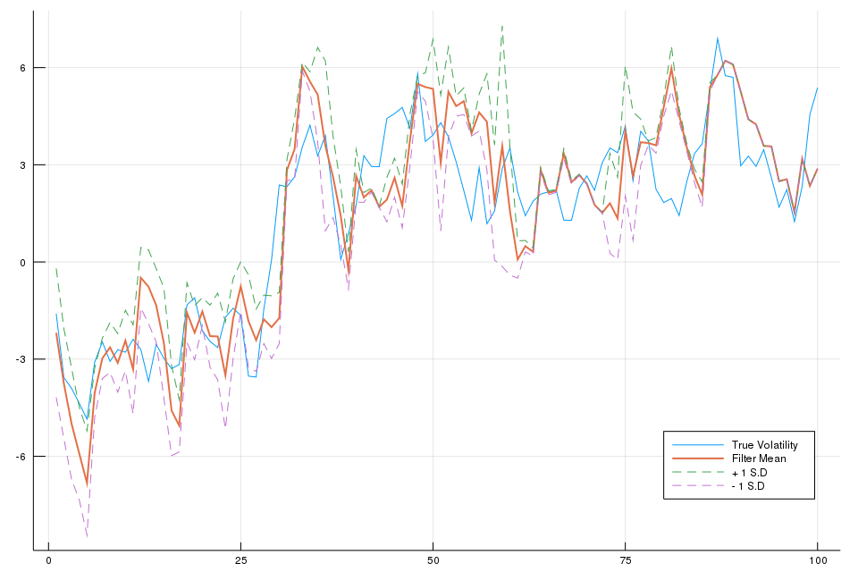
We obtain at time $n$

Apply the SIS algorithm (corresponding to the above SMC algorithm without a resampling step) with $N=1000$ particles, where we choose the proposal distribution as the conditional prior, then the particle weights are proportional to the likelihood function. At each time, the mean and standard deviation of $x_n$ conditional upon $y_{1:n}$ is estimated using the particle set, where the weights can represents the probability for discrete random variable. The detailed code is as follows:

# number of particles
N = 1000
X = ones(N, T)
W = ones(N, T)
μ = Normal(0, σ/sqrt(1-α^2))
f = x -> Normal(α*x, σ)
g = x -> Normal(0, β*sqrt(exp(x)))

xhat = ones(T)
xvar = ones(T)

for n = 1:T
    αn = ones(N)
    for i = 1:N
        # n = 1
        if n == 1
            X[i, 1] = rand(μ)
            W[i, 1] = pdf(g(X[i,1]), Y[1])
        else
            X[i, n] = rand(f(X[i,n-1]))
            αn[i] = pdf(g(X[i, n]), Y[n])
            W[i, n] = αn[i] * W[i, n-1]
        end 
    end
    W[:, n] .= W[:, n] / sum(W[:, n])
    xhat[n] = sum( X[:, n] .* W[:, n] )
    xvar[n] = sum( X[:, n].^2 .* W[:, n]) - xhat[n]^2
end

The I can use the following plotting code to reproduce Fig. 2 in the reference.

plot(x[1:100], label="True Volatility", legend = :bottomright, size = (960, 640))
plot!(xhat[1:100], label="Filter Mean", lw = 2)
plot!(xhat[1:100] .+ sqrt.(xvar[1:100]), label="+ 1 S.D", linestyle = :dash)
plot!(xhat[1:100] .- sqrt.(xvar[1:100]), label="- 1 S.D", linestyle = :dash)

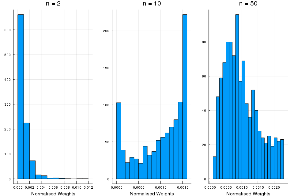
Also, we can plot the histograms of the particle weights at particular iteration:

p1 = histogram(W[:, 2]*1000, title = "n = 2", bins = 5, legend = false, xlabel = "Normalised Weights")
annotate!(28.0,0.0, L"\times 10^{-3}")
p2 = histogram(W[:, 10], title = "n = 10", xlims = (0, 1), bins = 5, legend = false, xlabel = "Normalised Weights")
p3 = histogram(W[:, 50], title = "n = 50", xlims = (0, 1), bins = 5, legend = false, xlabel = "Normalised Weights")
plot(p1, p2, p3, layout = (1,3), size = (960, 640))

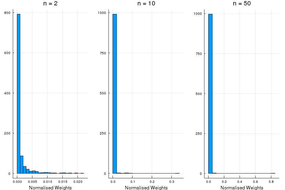
These histograms supports the theory that the failure of the SIS algorithm after a few iterations is due to weight degeneracy, showing that the number of particles with significant weight falls rapidly.

Considering multinomial resampling, I can implement the SMC for filtering as follows:

using StatsBase

for n = 1:T
    αn = ones(N)
    for i = 1:N
        # n = 1
        if n == 1
            X[i, 1] = rand(μ)
            W[i, 1] = pdf(g(X[i,1]), Y[1])
        else
            X[i, n] = rand(f(X[i,n-1]))
            αn[i] = pdf(g(X[i, n]), Y[n])
            W[i, n] = αn[i]
        end 
    end
    # resample
    idx = sample(1:N, weights(W[:, n]), N)
    X[:, 1:n] .= X[idx, 1:n]
    W[:, n] .= W[:, n] / sum(W[:, n])
    xhat[n] = sum( X[:, n] .* W[:, n] )
    xvar[n] = sum( X[:, n].^2 .* W[:, n]) - xhat[n]^2
end

The following figure shows that the algorithm does indeed produce a reasonable estimate and plausible credible interval.

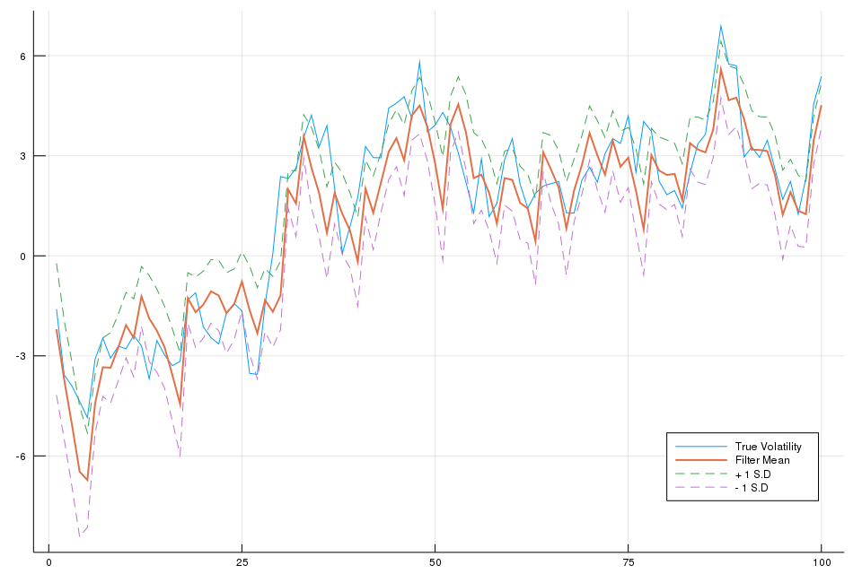
Similarly, the empirical distribution of particle weights for an SMC algorithm is

Auxiliary Particle Filtering

If importance weights are independent of the new state and the proposal distribution corresponds to the marginal distribution of the proposed state, then weighting, resampling and then sampling corresponds to a reweighting to correct for the discrepancy between the old and new marginal distribution of the earlier states, resampling to produce an unweighted sample and then generation of the new state from its condition distribution.

In a sense, the interchange of sampling and resampling is used to determine which particles should survive resampling at a given time.

It is desirable to find methods for making use of this future information in a more general setting, so that we can obtain the same advantage in situations in which it is not possible to make use of the optimal proposal distribution.

The Auxiliary Particle Filter (APF) is an alternative algorithm which does essentially this. The APF can be reinterpreted as a standard SMC algorithm applied to the following sequence of target distributions

with $\tilde p(y_{n+1}\mid x_n)$ chosen as an approximation of the predictive likelihood $p(y_{n+1}\mid x_n)$ if it is not known analytically. It follows that $\pi_n(x_{1:n})$ is an approximation of $p(x_{1:n}\mid y_{1:n+1})$ denoted $\tilde p(x_{1:n}\mid y_{1:n+1})$ given by

The associated incremental weight is given by

The APF proceeds as follows:

Auxiliary Particle Filtering

At time $n=1$

• Sample $X_1^i\sim q(x_1\mid y_1)$
• Compute the weights $w_1(X_1^i)=\frac{\mu(X_1^i)g(y_1\mid X_1^i)\tilde p(y_2\mid X_1^i)}{q(X_1^i\mid y_1)}$ and $W_1^i\propto w_1(X_1^i)$.
• Resample $\{W_1^i,X_1^i\}$ to obtain $N$ equally-weighted particles $\{\frac 1N, \bar X_1^i\}$.

At time $n\ge 2$

• Sample $X_n^i\sim q(x_n\mid y_n,\bar X_{n-1}^i)$ and set $X_{1:n}^i\leftarrow (\bar X_{1:n-1}^i,X_n^i)$.
• Compute the weights $\alpha_n(X_{n-1:n}^i)=\frac{g(y_n\mid X_n^i)f(X_n^i\mid X_{n-1}^i)\tilde p(y_{n+1}\mid X_n^i)}{\tilde p(y_n\mid X_{n-1}^i)q(X_n^i\mid y_n,X_{n-1}^i)}$ and $W_n^i\propto \alpha_n(X_{n-1:n}^i)$.
• Resample $\{W_n^i, X_{1:n}^i\}$ to obtain $N$ new equally-weighted particles $\{\frac 1N,\bar X_{1:n}^i\}$.

Note that this algorithm does not approximate the distributions $\{p(x_{1:n}\mid y_{1:n})\}$ but the distributions $\{\tilde p(x_{1:n}\mid y_{1:n+1})\}$, we use IS to obtain an approximation of $p(x_{1:n}\mid y_{1:n})$ with

as the importance distribution. A Monte Carlo approximation of this importance distribution is obtained after the sampling step in the APF and the associated unnormalised importance weights are given by

It follows that we obtain

where $\tilde W_n^i\propto \tilde w_n(X_{n-1:n}^i)$.

Limitations of Particle Filters

1. Even if the optimal importance distribution $p(x_n\mid y_n,x_{n-1})$ can be used, this doesn’t guarantee that the SMC algorithms will be efficient.
2. If resampling very frequently, the particle approximation $\hat p(x_{1:n}\mid y_{1:n})$ of the joint distribution $p(x_{1:n}\mid y_{1:n})$ will be unreliable.
3. Only the variables $\{X_n^i\}$ are sampled at time $n$ but the path values $\{X_{1:n-1}^i\}$ remain fixed.

Resample-Move

Whilst MCMC uses Markov kernels with appropriate invariant distributions to generate collections of correlated samples, the Resample-Move algorithm uses them within an SMC algorithm as a principled way to “jitter” the particle locations and thus to reduce degeneracy.

SMC Filtering with MCMC Moves

At time $n=1$

• Sample $X_1^i\sim q(x_1\mid y_1)$
• Compute the weights $w_1(X_1^i)=\frac{\mu(X_1^i)g(y_1\mid X_1^i)}{q(X_1^i\mid y_1)}$ and $W_1^i\propto w_1(X_1^i)$
• Resample $\{W_1^i, X_1^i\}$ to obtain $N$ equally-weighted particles $\{\frac 1N, \bar X_1^i\}$.
• Sample $X_1’^i\sim K_1(x_1\mid \bar X_1^i)$

At time $1 < n < L$

• Sample $X_n^i\sim q(x_n\mid y_n)$ and set $X_{1:n}^i\leftarrow (X_{1:n-1}’^i, X_n^i)$
• Compute the weights $\alpha_n(X_{n-1:n}^i)=\frac{g(y_n\mid X_n^i)f(X_n^i\mid X_{n-1}^i)}{q(X_n^i\mid y_n,X_{n-1}^i)}$ and $W_n^i\propto \alpha_n(X_{n-1:n}^i)$.
• Resample $\{W_n^i, X_{1:n}^i\}$ to obtain $N$ equally-weighted particles $\{\frac 1N, \bar X_{1:n}^i\}$
• Sample $X_{1:n}’^i\sim K_n(x_{1:n}\mid \bar X_{1:n}^i)$

At time $n\ge L$

• Sample $X_n^i\sim q(x_n\mid y_n)$ and set $X_{1:n}^i\leftarrow (X_{1:n-1}’^i, X_n^i)$
• Compute the weights $\alpha_n(X_{n-1:n}^i)=\frac{g(y_n\mid X_n^i)f(X_n^i\mid X_{n-1}^i)}{q(X_n^i\mid y_n,X_{n-1}^i)}$ and $W_n^i\propto \alpha_n(X_{n-1:n}^i)$.
• Resample $\{W_n^i, X_{1:n}^i\}$ to obtain $N$ equally-weighted particles $\{\frac 1N, \bar X_{1:n}^i\}$
• Sample $X_{n-L+1:n}’^i\sim K_n(x_{n-L+1:n}\mid \bar X_{1:n}^i)$ and set $X_{1:n}’^i\leftarrow (\bar X_{1:n-L}^i, X_{n-L+1:n}’^i)$

Block Sampling

Although the resample-move allow us to reintroduce some diversity among the set of particles after the resampling step over a lag of length $L$, the importance weights have the same expression as for the standard particle filter. So this strategy does not significantly decrease the number of resampling steps compared to a standard approach.

An alternative block sampling goes further than the resample-move method, which aims to sample only the components $x_n$ at time $n$ in regions of high probability mass and then to uses MCMC moves to rejuvenate $x_{n-L+1:n}$ after a resampling step. The block sampling algorithm attempt to directly sample the components $x_{n-L+1:n}$ at time $n$; the previously-sampled values of the components $x_{n-L+1:n-1}$ sampled are simply discarded.

SMC Block Sampling for Filtering

At time $n=1$

• Sample $X_1^i\sim q(x_1\mid y_1)$
• Compute the weights $w_1(X_1^i)=\frac{\mu(X_1^i)g(y_1\mid X_1^i)}{q(X_1^i\mid y_1)}$ and $W_1^i\propto w_1(X_1^i)$.
• Resample $\{W_1^i,X_1^i\}$ to obtain $N$ equally-weighted particles $\{\frac 1N, \bar X_1^i\}$

At time $1< n <L$

• Sample $X_{1:n}^i\sim q(x_{1:n}\mid y_{1:n})$
• Compute the weights $\alpha_n(X_{1:n}^i)=\frac{p(X_{1:n}^i,y_{1:n})}{q(X_{1:n}^i\mid y_{1:n})}$ and $W_n^i\propto \alpha_n(X_{n-1:n})$ (???)
• Resample $\{W_n^i,X_{1:n}^i\}$ to obtain $N$ equally-weighted particles $\{\frac 1N, \bar X_{1:n}^i\}$.

At time $n\ge L$

• Sample $X_{n-L+1:n}^i\sim q(x_{n-L+1:n}\mid y_{n-L+1:n},\bar X_{1:n-1}^i)$
• Compute the weights $w_n(\bar X_{n-L:n-1},X_{n-L+1:n}^i)$ and $W_n^i\propto w_n(\cdot)$.
• Resample $\{W_n^i,\bar X_{1:n-L}^i, X_{n-L+1:n}^i\}$ to obtain $N$ new equally weighted particles $\{\frac 1N, \bar X_{1:n}^i\}$.

Rao-Blackwellised Particle Filtering

“A good Monte Carlo is a dead Monte Carlo”. Whenever an integral can be calculated analytically doing so should be preferred to the use of Monte Carlo techniques.

Assume that one is interested in sampling from $\pi(x)$ with $x=(u,z)\in\cU\times \cZ$ and

where $\pi(u)=Z^{-1}\gamma(u)$ and

admits a close-form expression. Then if we are interested in approximating $\pi(x)$ and computing $Z$, we only need to perform a MC approximation $\pi(u)$ and $Z=\int \gamma(u)du$ on the space $\cU$ instead of $\cU\times \cZ$.

Two classes of important models where this simple idea can be used successfully:

• Conditionally linear Gaussian models
• Partially observed linear Gaussian models

Particle Smoothing

SMC methods can provide an approximation of the sequence of distributions $\{p(x_{1:n},y_{1:n})\}$. Consequently, sampling from a joint distribution $p(x_{1:T},y_{1:T})$ and sample from/marginalize SMC approximation $\hat p(x_{1:T},y_{1:T})$ to approximate the marginals $\{p(x_n\mid y_{1:T})\}$ for $n=1,\ldots,T$.

But this approach is bound to be inefficient when $T$ is large as the successive resampling steps leas to particle degeneracy: $\hat p(x_{1:n}\mid y_{1:T})$ is approximated by a single unique particle for $n«T$.

Fixed-lag Approximation

For HMM with “good” forgetting properties,

for $\Delta$ large enough; that is observations collected at times $k > n+\Delta$ do not bring any additional information about $x_{1:n}$. We need to replace $\Delta$ with an estimate of it denoted $L$. Note that such fixed-lag SMC schemes do not converge asymptotically towards the true smoothing distributions because we do not have $p(x_{1:n}\mid y_{1:T})=p(x_{1:n}\mid y_{1:\min(n+L,p)})$. However, the bias might be negligible and can be upper bounded under mixing conditions.

Forward Filtering-Backward Smoothing

It is possible to sample from $p(x_{1:T}\mid y_{1:T})$ and compute the marginals $\{p(x_n\mid y_{1:T})\}$ using forward-backward formula.

Generalized Two-Filter Formula

To obtain an SMC approximation of the generalised two-filter formula, we need to approximate the backward filter $\{\tilde p(x_n\mid y_{n:T})\}$ and to combine the forward filter and the backward filter in a sensible way.

Summary

Advantages for interpreting all of these algorithms as particular cases of the general algorithm:

• The standard algorithm may be viewed as a particle interpretation of a Feynman-Kac model and hence strong, sharp theoretical results can be applied to all algorithms within this common formulation.
• By considering all algorithms within the same framework it is possible to develop a common understanding and intuition allowing meaningful comparisons to be drawn and sensible implementation decisions to be made.

Limitations and problems:

• for sufficiently high-dimensional spaces and sufficiently complex distributions, it is impossible to obtain an accurate characterisation in a reasonable amount of time.
• estimate the vector of parameters
• although some algorithms, it cannot be considered to have been solved in full generality.