Theoretical Results of Lasso

Posted on Mar 26, 2019 (Update: Jan 16, 2020)

Tags: Lasso, Sparsistency, Strong Convexity, Restricted Eigenvalues, Cone Constraint, Mutual Incoherence

Prof. Jon A. WELLNER introduced the application of a new multiplier inequality on lasso in the distinguish lecture, which reminds me that it is necessary to read more theoretical results of lasso, and so this is the post, which is based on Hastie, T., Tibshirani, R., & Wainwright, M. (2015). Statistical Learning with Sparsity. 362.

Introduction

Consider the standard linear regression model in matrix-vector form,

\begin{equation} \y = \X\beta^* +\w\label{eq:model} \end{equation}

this post focuses on some theoretical guarantees for both the constrained form of the lasso

\[\min_{\Vert \beta\Vert_1\le R}\Vert \y-\X\beta\Vert^2_2\,,\]

as well as for its Lagrangian version

\[\min_{\beta\in\bbR^p}\{\frac{1}{2N}\Vert \y-\X\beta\Vert^2_2 + \lambda_N\Vert \beta\Vert_1\}\]

Types of Loss Functions

• Prediction loss function: \(\cL{\pred}(\hat\beta;\beta^*) = \frac 1N \Vert \X\hat\beta-\X\beta^*\Vert_2^2\)
• Parameter estimation loss: \(\cL_2(\hat\beta;\beta^*)=\Vert \hat\beta-\beta^*\Vert_2^2\)
• Variable selection or Support recovery: \(\cL_{\vs}(\hat\beta;\beta^*) = \begin{cases} 0 & \text{ if }\sign(\hat\beta_i) = \sign(\beta_i^*)\text{ for all }i=1,\ldots,p\\ 1 & \text{ otherwise} \end{cases}\)

Types of Sparsity Models

Aims to develop theory that is applicable to the high-dimensional regime, meaning that it allows for the scaling $p \ge N$.

Whenever $N < p$, the linear model \eqref{eq:model} is unidentifiable(there exist $\beta_1\neq \beta_2$ for which $\X\beta_1=\X\beta_2$); for instance, it is impossible to distinguish between the models $\beta^*=0$ and $\beta^*=\Delta$, where $\Delta=\bbR^p$ is any element of the $p-N$ dimensional nullspace of $\X$.

For this reason, it is necessary to impose additional constraints on the unknown regression vector $\beta^*\in\bbR^p$.

• hard sparsity: $\beta^*$ has at most $k \le p$ nonzero entries.
• weakly sparsity: $\beta^*$ can be closely approximated by vectors with few nonzero entries. One way of formalizing this notion is by defining the $\ell_q$-“ball” of radius $R_q$,

\[\bbB(R_q) = \{\beta\in\bbR^p\mid \sum_{j=1}^p\vert \beta_i\vert^q\le R_q\}\,.\]

In the special case $q=0$, imposing the constraint $\beta^*\in \bbB(R_0)$ is equivalent to requiring that $\beta^*$ has at most $k=R_0$ nonzero entries.

Bounds on Lasso $\ell_2$-Error

Focus on the case when $\beta^*$ is $k$-sparse, meaning that its entries are nonzero on a subset $S(\beta^*)\subset\{1,2,\ldots,p\}$ of cardinality $k=\vert S(\beta^*)\vert$.

Strong Convexity in the Classical Setting

Begin by developing some conditions on the model matrix $\X$ that are needed to establish bounds on $\ell_2$-error. In order to provide some intuition for these conditions, consider one route for proving $\ell_2$-consistency in the classical setting ($p$ fixed, $N$ tending to infinity).

Suppose that the difference in function values $\Delta f_N=\vert f_N(\hat\beta)-f_N(\beta^*)\vert$ converges to zero as the sample size $N$ increases. The key question is what additional conditions are needed to ensure that the $\ell_2$ norm of the parameter vector difference $\Delta\beta=\Vert \hat\beta-\beta^*\Vert_2$ also converges to zero?

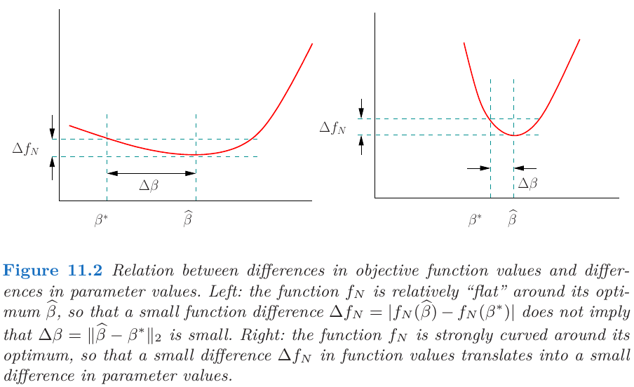
A natural way to specify that a function is suitably “curved” is via the notion of strong convexity. Given a differentiable function $f:\bbR^p\rightarrow \bbR$, it is strongly convex with parameter $\gamma > 0$ at $\theta\in \bbR^p$ if the inequality

\[f(\theta') - f(\theta)\ge \nabla f(\theta)^T(\theta'-\theta) + \frac{\gamma}{2}\Vert \theta'-\theta\Vert_2^2\]

hold for all $\theta’\in \bbR^p$.

The following conditions are all equivalent to the condition that a differentiable function $f$ is strongly convex with constant $\mu > 0$.

1. $f(y) \ge f(x) + \nabla f(x)^T(y-x) + \frac{\mu}{2}\Vert y-x\Vert^2, \forall x, y$.
2. $g(x) = f(x) - \frac{\mu}{2}\Vert x\Vert^2$ is convex for all $x$.
3. $(\nabla f(x) - \nabla f(y))^T(x-y) \ge \mu\Vert x-y\Vert^2, \forall\; x,y$.
4. $f(\alpha x+(1-\alpha)y)\le \alpha f(x) + (1-\alpha)f(y) - \frac{\alpha(1-\alpha)\mu}{2}\Vert x-y\Vert^2, \alpha\in[0,1]$.

For a continuously differentiable function $f$, the following conditions are all implied by strong convexity (SC) condition.

1. $\frac 12\Vert\nabla f(x)\Vert^2 \ge \mu\Vert f(x) - f^*\Vert,\forall x$.
2. $\Vert \nabla f(x)-\nabla f(y)\Vert \ge \mu\Vert x-y\Vert, \forall x, y$
3. $f(y)\le f(x)+\nabla f(x)^T(y-x)+\frac{1}{2\mu}\lVert\nabla f(y)- \nabla f(x)\rVert^2,~\forall x,y.$
4. $(\nabla f(x) - \nabla f(y)^T(x-y) \le \frac{1}{\mu} \lVert\nabla f(x)-\nabla f(y)\rVert^2, ~\forall x,y.$

Actually, if $f$ is convex, then Proposition 1(3) is equivalent to Proposition 2(2), as proved in Proof to a criterion of strongly convexity – Yanjun Han.

Alexandrov theorem states that if $U$ is an open set of $\bbR^p$ and $f:U\rightarrow \bbR^m$ is a convex function, then $f$ has a second derivative almost everywhere. Proposition 1(3) implies that $\nabla^2f(x)\succeq mI$. Now for any fixed $x, y$, define

\[g_n(t) = n(y-x)^T(\nabla f(x+t(y-x)+(y-x)/n) - \nabla f(x+t(y-x)) )\]

for $t\in [0, 1-1/n]$, and $g_n(t) = 0$ for $t = (1-1/n, 1]$. Then

\[\lim\inf g_n(t) = (y-x)^TD_{y-x}\nabla f(x+t(y-x)) = (y-x)^T\nabla^2f(x+t(y-x))(y-x)\,,\]

where $D_{y-x}$ denotes the directional derivative, and note that $g_n\ge 0$ (by the monotonicity of gradient for convexity), Fatou’s lemma yields

\[m\Vert y-x\Vert_2^2 \le \int_0^1\lim\inf g_n(t)dt \le\lim\inf\int_0^1 g_n(t)dt = (y-x)^T(\nabla f(y)-\nabla f(x))\]

I am confused that the original proof still have one term $\lim\sup \int_0^{1/n}$.

But if $f$ is not convex, there are counterexamples that Proposition 2(2) holds but Proposition 1(3) fails, such as $f(x) = -x^2$ mentioned in Xingyu Zhou’s response to a comment.

An alternative characterization of strong convexity is in terms of the Hessian $\nabla^2 f$: in particular, the function $f$ is strongly convex with parameter $\gamma$ around $\beta^*$ iff the minimum eigenvalue of the Hessian matrix $\nabla^2f(\beta)$ is at least $\gamma$ for all vectors $\beta$ in a neighborhood of $\beta^*$.

If $f$ is the negative log-likelihood under a parametric model, then $\nabla^2 f(\beta^*)$ is the observed Fisher information matrix, so that strong convexity corresponds to a uniform lower bound on the Fisher information in all directions.

Restricted Eigenvalues for Regression

In high-dimensional setting, it is clear that the least-squares objective function $f_N(\beta) = \frac{1}{2N}\Vert \y-\X\beta\Vert_2^2$ is always convex; under what additional conditions is it also strongly convex? Simple calculation yields $\nabla^2 f(\beta)=\X^T\X/N$ for all $\beta\in\bbR^p$. Thus, the least squares loss is strongly convex iff the eigenvalues of the $p\times p$ positive semidefinite matrix $\X^T\X$ are uniformly bounded away from zero. But now $\X^T\X$ has rank at most $\min\{N,p\}$, so it is always rank-deficient, and hence not strongly convex.

For this reason, to relax the notion of strong convexity. A function $f$ satisfies restricted strong convexity at $\beta^*$ w.r.t. $\cC$ if there is a constant $\gamma > 0$ such that

\[\frac{\nu^T\nabla^2f(\beta)\nu}{\Vert \nu\Vert_2^2}\text{ for all nonzero }\nu\in\cC\,,\]

and for all $\beta\in\bbR^p$ in a neighborhood of $\beta^*$. In the linear regression, this notion is equivalent to lower bounding the restricted eigenvalues of the model matrix,

\[\frac{\frac 1N\nu^T\X^T\X\nu}{\Vert\nu\Vert_2^2}\ge \gamma\text{ for all nonzero }\nu\in\cC\,.\]

Suppose $\beta^*$ is sparse, supported on the subset $S=S(\beta^*)$. Defining the lasso error $\hat\nu = \hat\beta-\beta^*$, let $\hat\nu_S\in \bbR^{\vert S\vert}$ denote the subvector indexed by elements of $S$, similarly for $\hat\nu_{S^c}$. For appropriate choices of the $\ell_1$-ball radius, or equivalently, the regularization parameter $\lambda_N$, it turns out that the lasso error satisfies a cone constraint of the form

\[\Vert \hat\nu_{S^c}\Vert_1\le \alpha\Vert \hat\nu_S\Vert_1\,,\]

for some constant $\alpha \ge 1$. Thus, the lasso error is restricted to a set of the form

\[\cC(S;\alpha):=\{\nu\in \bbR^p\vert \Vert \nu_{S^c}\Vert_1\le \alpha\Vert \nu_S\Vert_1\}\,,\]

for some parameter $\alpha\ge 1$.

Prof. Jon A. WELLNER mentioned a similar notion, the so-called compatibility condition: For any $L > 0$ and $S\subset\{1,\ldots,d\}$, define

\(\phi(L,S)= \sqrt{\vert S\vert}\min \left\{\frac{1}{\sqrt n}\Vert X\theta_S-X\theta_{S^c}\Vert_2:\Vert\theta_S\Vert_1=1,\Vert \theta_{S^c}\Vert_1\le L\right\}\).

A Basic Consistency Result

Bounds on Prediction Error

Support Recovery in Linear Regression

Given an optimal lasso solution $\hat\beta$, when is its support set $\hat S=S(\hat\beta)$ exactly equal to the true support $S$? This property is referred as variable selection consistency or sparsistency.

Variable-Selection Consistency for the Lasso

Variable selection requires a condition related to but distinct from the restricted eigenvalue condition. Assume a condition know either as mutual incoherence or irrepresentability: there must exist some $\gamma > 0$ such that

\[\max_{j\in S^c}\Vert (\X_S^T\X_S)^{-1}\X_S^T\x_j \Vert_1\le 1-\gamma\,.\]

Also assume that the design matrix has normalized columns

\[\max_{j=1,\ldots,p}\Vert \x_j\Vert_2/\sqrt N \le K_\mathrm{clm}\,.\]

Further assume that the submatrix $\X_S$ is well-behaved in the sense that

\[\lambda_\min(\X_S^T\X_S/N)\ge C_\min\,.\]

References

• Zhou, Xingyu. “Strong convexity”.