Studentized U-statistics
Posted on
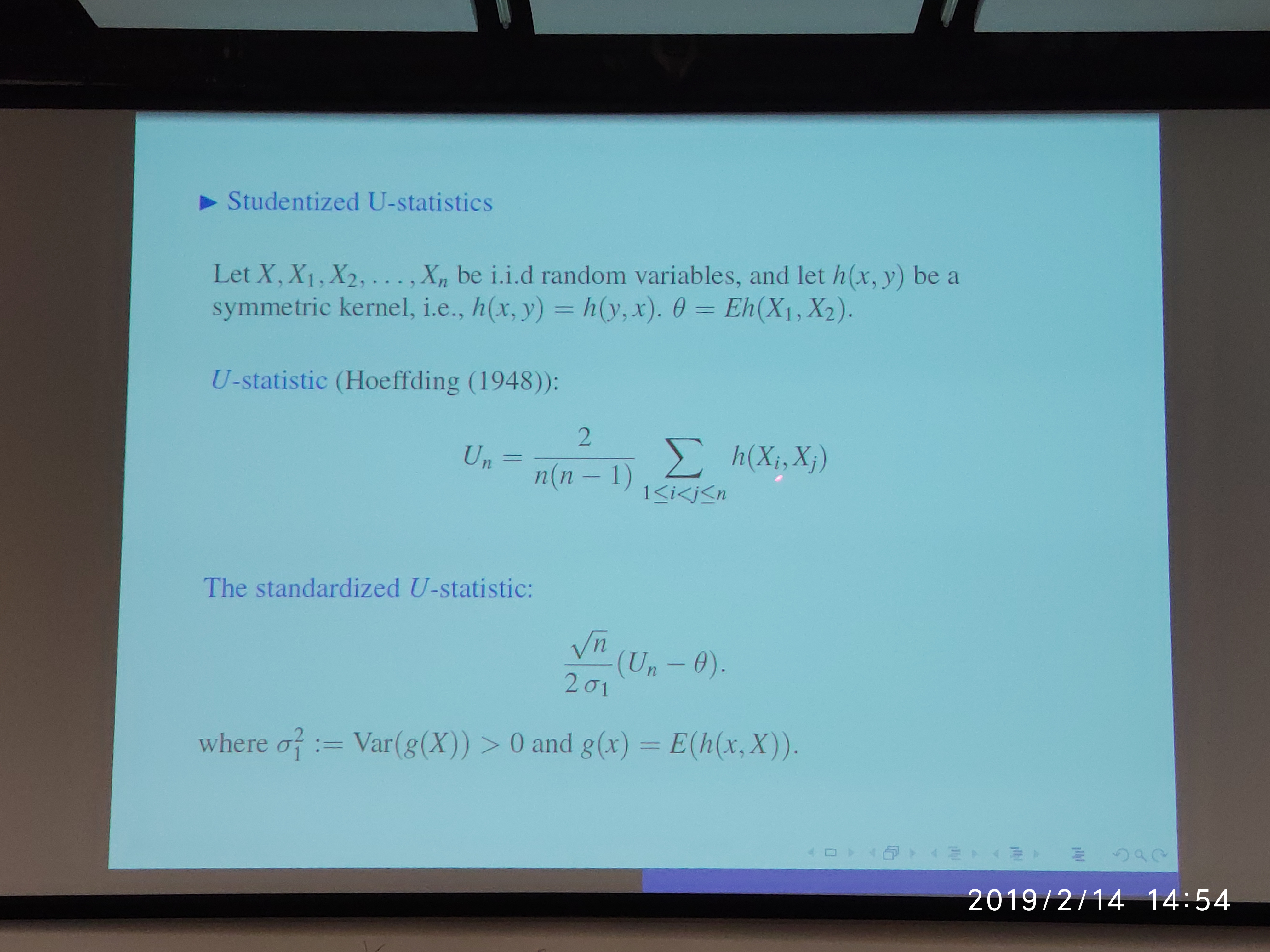
In Prof. Shao’s wonderful talk, Wandering around the Asymptotic Theory, he mentioned the Studentized U-statistics. I am interested in the derivation of the variances in the denominator.

Consider the U-statistic,
\[\begin{equation} U_n = \binom{n}{m}^{-1}\sum_{C_n} h(X_{\alpha_1},\ldots,X_{\alpha_m})\,, \label{eq:udef} \end{equation}\]where $\sum_{C_n}$ denotes the summation over the $\binom{n}{m}$ combinations of $m$ distinct elements $\{\alpha_1,\ldots,\alpha_m\}$ from $\{1,\ldots,n\}$.
Standardized Form
The Hoeffding’s Theorem can be used to calculate the variance of $U_n$:
For $m=2$,
\[\begin{align*} \Var(U_n) &= \binom{n}{2}^{-1}\sum_{k=1}^2\binom{2}{k}\binom{n-2}{2-k}\zeta_k\\ &=\frac{2}{n(n-1)}\Big(2(n-2)\zeta_1+\zeta_2\Big)\,, \end{align*}\]where $\zeta_1=\Var(h_1(X_1))$ and $\zeta_2 = \Var(h_2(X_1,X_2))$. Note that
\[\begin{align*} h_1(x_1) &= \E[h(x_1, X)] \triangleq g(x_1)\\ h_2(x_1,x_2) &= \E[h(x_1, x_2)] = h(x_1,x_2)\,, \end{align*}\]thus,
\[\Var(U_n) = \frac{2}{n(n-1)}\Big(2(n-2)\Var(g(X_1))+\Var(h(X_1,X_2))\Big)\,,\]which is similar to the standardized term $\frac{4\Var(g(X_1))}{n}$ in the slide except the extra term $\zeta_2$ and an additional coefficient $\frac{n-2}{n-1}$ for $\zeta_1$.
Let us resort to the asymptotic result (Jun Shao, 2003):
Now for the special case $m=2$, we have
\[h_1(x_1) = \E[h(x_1, X)] \triangleq g(x_1)\,,\]then the standardized form is
\[\frac{\sqrt{n}(U_n-\theta)}{\sqrt{4\xi_1}} =\frac{\sqrt{n}(U_n-\theta)}{2\sqrt{\Var(g(X))}} = \frac{\sqrt{n}(U_n-\theta)}{2\sigma_1}\,.\]Studentized Form
Arvesen, J. N. (1969) considers the jackknife estimate, define
\[U_n^{\backslash k} = \binom{n-1}{m}^{-1}\sum_{C_n^{\backslash k}}h(X_{\beta_1^{\backslash k}},\ldots, X_{\beta_m^{\backslash k}})\,,\]where $C^{\backslash k}_{n-1}$ indicates that the summation is over all combinations $(\beta_1^{\backslash k},\ldots, \beta_m^{\backslash k})$ of $m$ integers chosen from $(1,\ldots,k-1,k+1,\ldots, n)$.
Arvesen, J. N. (1969) proves that
\[\begin{equation} (n-1)\sum_{k=1}^n(U_n^{\backslash k}-U_n)^2\rightarrow m^2\zeta_1\,. \label{eq:approx} \end{equation}\]For $m=2$, we have
\[\begin{align*} (n-1)\sum_{k=1}^n(U_n^{\backslash k}-U_n)^2 &= (n-1)\sum_{k=1}^n\Big(\frac{2}{(n-1)(n-2)}\sum_{i< j;\,, i,j\neq k}h(X_i,X_j)-U_n\Big)^2\\ & = \frac{4(n-1)}{(n-2)^2}\sum_{k=1}^n\Big(\frac{1}{n-1}\sum_{i < j;\,, i,j\neq k}h(X_i,X_j)-\frac{n-2}{2}U_n\Big)^2\\ & \rightarrow 4\zeta_1\,, \end{align*}\]which implies that
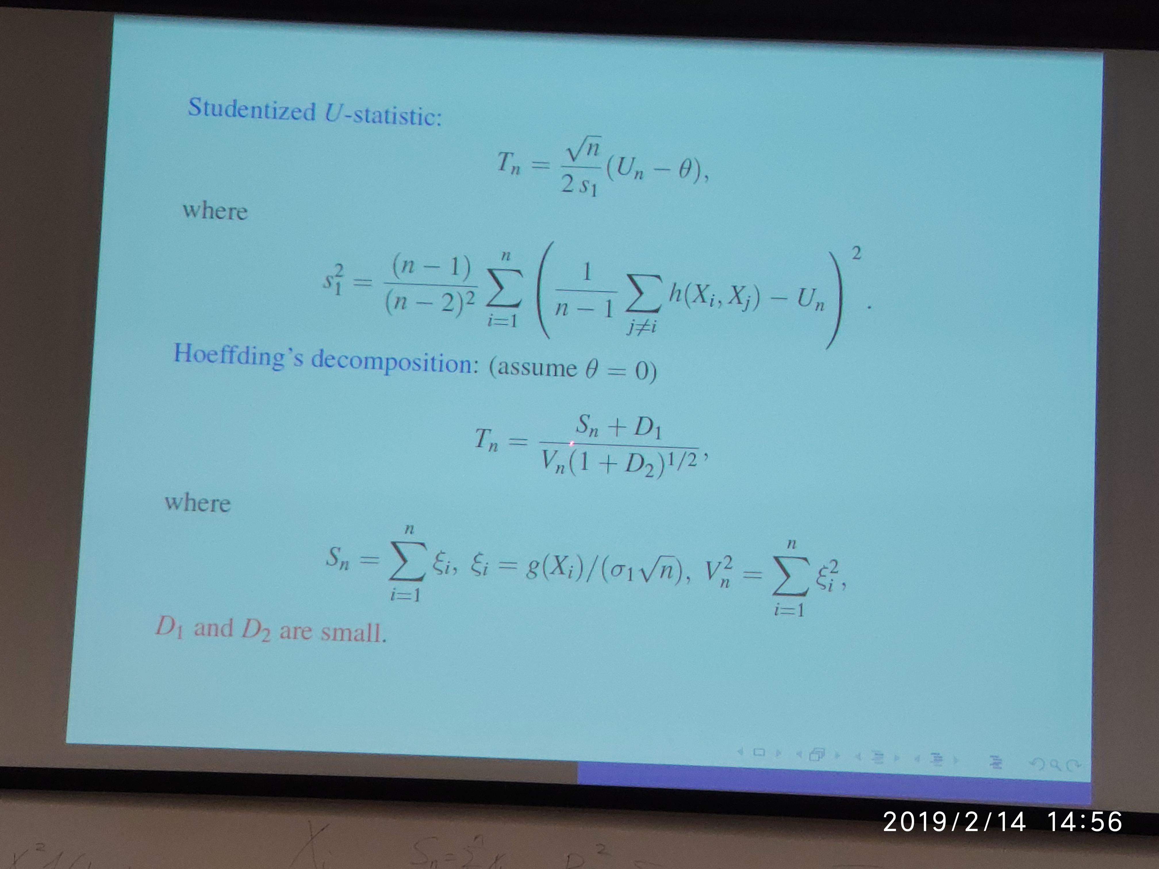
\[\begin{equation} s^2_* \triangleq \frac{(n-1)}{(n-2)^2}\sum_{k=1}^n\Big(\frac{1}{n-1}\sum_{i < j;\,, i,j\neq k}h(X_i,X_j)-\frac{n-2}{2}U_n\Big)^2\rightarrow \zeta_1=\sigma_1^2\,. \label{eq:sstar} \end{equation}\]But in the following slide,

$s_*^2$ and $s_1^2$ are too different, only share the same coefficient.
I am confused, and asked help from Prof. Shao, he explained that there are various definitions of jackknife estimate, which means that it is also possible to construct other approximations different from $\eqref{eq:approx}$, and the Studentized form in the slide can be viewed as only keeping $X_i$ in each “jackknife”, i.e., the summation is over $(i, j)$, where $i$ is fixed, $j$ is chosen from $(1,\ldots,i-1,i+1,\ldots,n)$.
However, I haven’t discuss more details with Prof. Shao, and I am still curious about the derivation of variance in the Jackknife form, and want to know if it is possible to work further with $\eqref{eq:sstar}$.