Cox Models with Time-Varying Covariates vs Time-Varying Coefficients
Posted on
The classical Cox model is
\[\lambda(t\mid X) = \lambda_0(t)\exp(\beta^TX)\,,\]one approach for using time-varying covariate data is to extend the Cox model to allow time-varying covariates
\[\lambda(t\mid Z(t)) = \lambda_0(t) \exp(\beta^Tx +\gamma^TXg(t))\]where
\[Z(t) = [x_1,\ldots,x_p, X_1g(t),\ldots, X_qg(t)]\]In the time-varying coefficient situation, a covariate is measured at baseline but its effect on the outcome is not constant over the follow-up time, which is a violation of the proportional hazards assumption.
If the time-varying coefficient can be written as $g(\beta, t) = \beta g(t)$, the model with a time-varying coefficient can be expressed as a model with time-varying covariate with a constant coefficient.
Working example on time-varying covariates
generate a data frame containing two time-fixed variables: group and age
library(survsim)
library(survival)
N = 100
set.seed(123)
df.tf = simple.surv.sim(
  n = N, foltime = 500,
  dist.ev = c("llogistic"),
  anc.ev = c(0.68),
  beta0.ev = c(5.8),
  anc.cens = 1.2,
  beta0.cens = 7.4,
  z = list(c("unif", 0.8, 1.2)),
  beta = list(c(-0.4), c(0)),
  x = list(c("bern", 0.5), c("normal", 70, 13))
)
names(df.tf)[c(1, 6, 7)] = c("id", "grp", "age")
head(df.tf)
#   id status start      stop         z grp      age
# 1  1      1     0  48.12817 1.1532070   0 80.40721
# 2  2      0     0 121.43904 0.9826459   1 86.11345
# 3  3      1     0  30.65770 1.1599300   1 72.38007
# 4  4      0     0 500.00000 1.0771214   0 91.97240
# 5  5      1     0  69.54117 1.0376568   1 77.13826
# 6  6      1     0 233.05486 1.1181870   1 86.83192
construct a time-varying covariate crp, generate a data frame in a counting process data structure, in which each individual is represented by one or more rows. In such a data frame, each row represents a follow-up tine interval at which the value of a covariate is recorded.
set.seed(123)
nft = sample(1:10, N, replace = TRUE)
crp = round(abs(rnorm(sum(nft)+N, mean = 100, sd = 40)), 1)
time = NULL
id = NULL
i = 0
for (n in nft) {
  i = i+1
  time.n = sample(1:500, n)
  time.n = c(0, sort(time.n))
  time = c(time, time.n)
  id.n = rep(i, n+1)
  id = c(id, id.n)
}
df.td = cbind(data.frame(id, time), crp)
head(df.td)
> head(df.td)
#   id time   crp
# 1  1    0 115.4
# 2  1  207  85.2
# 3  1  253 125.8
# 4  1  373  91.2
# 5  2    0 113.3
# 6  2  110 143.9
Merging data frames via tmerge
# convert the data frame to a longitudinal type. the first run defining the basic structure
# and subsequent runs add variables to that structure
df = tmerge(df.tf, df.tf, id = id, endpt = event(stop, status))
head(df)
#   id status start      stop         z grp      age tstart     tstop endpt
# 1  1      1     0  48.12817 1.1532070   0 80.40721      0  48.12817     1
# 2  2      0     0 121.43904 0.9826459   1 86.11345      0 121.43904     0
# 3  3      1     0  30.65770 1.1599300   1 72.38007      0  30.65770     1
# 4  4      0     0 500.00000 1.0771214   0 91.97240      0 500.00000     0
# 5  5      1     0  69.54117 1.0376568   1 77.13826      0  69.54117     1
# 6  6      1     0 233.05486 1.1181870   1 86.83192      0 233.05486     1
df = tmerge(df, df.td, id = id, crp = tdc(time, crp))
head(df)
#   id status start      stop         z grp      age tstart     tstop endpt   crp
# 1  1      1     0  48.12817 1.1532070   0 80.40721      0  48.12817     1 115.4
# 2  2      0     0 121.43904 0.9826459   1 86.11345      0 110.00000     0 113.3
# 3  2      0     0 121.43904 0.9826459   1 86.11345    110 121.43904     0 143.9
# 4  3      1     0  30.65770 1.1599300   1 72.38007      0  30.65770     1 146.0
# 5  4      0     0 500.00000 1.0771214   0 91.97240      0  18.00000     0  71.6
# 6  4      0     0 500.00000 1.0771214   0 91.97240     18 366.00000     0 110.3
Fit the Cox model with a time-varying covariate
# fit the cox model with a time-varying covariate
fit.tdc = coxph(Surv(tstart, tstop, endpt)~grp+age+crp+cluster(id), df)
fit.tdc
Time-varying coefficients.
It emerges when the proportional hazards assumption is not fulfilled to identify time-varying coefficients is actually to test the proportional hazards assumption after fitting a Cox proportional hazard model.
The examination of proportional hazards assumption can be performed using cox.zph() function, shipped with the survival package
fit2 = coxph(Surv(time, status) ~ age + ph.karno + sex, data = lung)
zph = cox.zph(fit2)
zph
#           chisq df      p
# age       0.478  1 0.4892
# ph.karno  8.017  1 0.0046
# sex       3.085  1 0.0790
# GLOBAL   10.359  3 0.0157
Schoenfeld’s global test for the violation of proportional assumption
The result shows that there is significant deviation from the proportional hazards assumption for the variable pb.karno
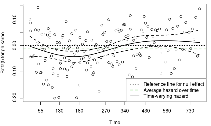
We can visualize the results
plot(zph[2], lwd = 2)
abline(0, 0, col = 1, lty = 3, lwd = 2)
abline(h = fit2$coef[2], col = 3, lwd = 2, lty = 2)
legend("bottomright",
       legend=c("Reference line for null effect",
                "Average hazard over time",
                "Time-varying hazard"),
       lty = c(3, 2, 1), col = c(1, 3, 1), lwd = 2)
Step function to explore time-varying coefficient
one way to model time-varying coefficients is to use a step function, the effect of fixed baseline covariates becomes stronger or weaker over time, which can be explored via stratification by time
lung.split = survSplit(Surv(time, status) ~ .,
                       data = lung, cut = c(180, 350),
                       episode = "tgroup", id = "id")
fit.split = coxph(Surv(tstart, time, status) ~ age + ph.karno:strata(tgroup) +
                    sex, data = lung.split)
cox.zph(fit.split)
#                            chisq df    p
# age                     0.000321  1 0.99
# sex                     2.531266  1 0.11
# ph.karno:strata(tgroup) 4.840271  3 0.18
# GLOBAL                  7.315512  5 0.20
Continuous function to describe the time-varying coefficient
## continuous function to describe the time-varying coefficient
fit.tt = coxph(Surv(time, status) ~ age+ph.karno+tt(ph.karno)+sex, data = lung, tt = function(x, t,...) x*log(t+20))

zph.tt = cox.zph(fit2, transform = function(t) log(t+20))
plot(zph.tt[2])
abline(coef(fit.tt)[2:3], col=2)
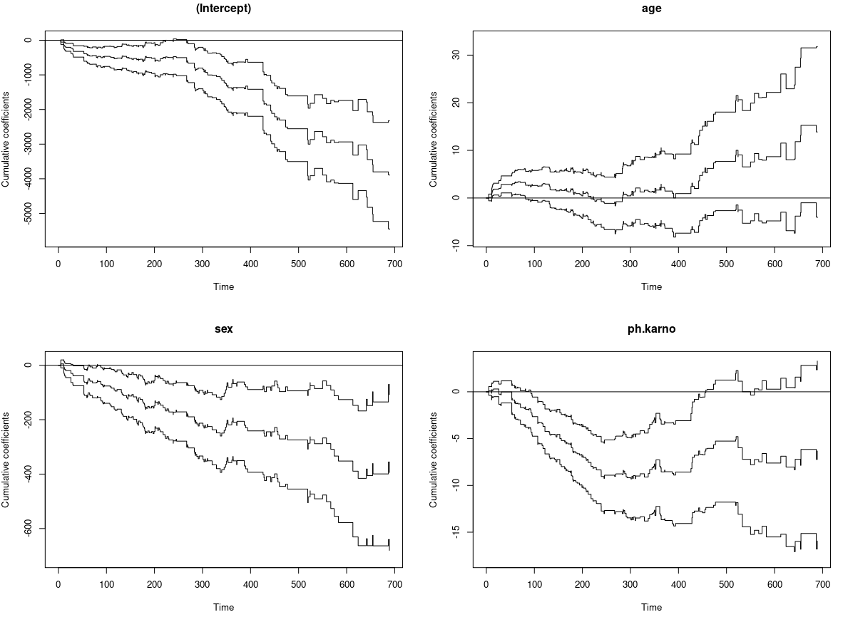
timereg package
Cox regression model is fit similarly as in the survival package with the only difference that resampling methods are used for the statistical inference
library(timereg)
fit.out = timecox(Surv(time, status) ~ age+sex+ph.karno, data = lung, n.sim = 500, max.time = 700)

# the effects of all variables
par(mfrow = c(2, 2))
plot(fit.out)