Bayesian Hierarchical Varying-Sparsity Regression Models with Application to Cancer Proteogenomics.
Posted on
propose Bayesian hierarchical varying-sparsity regression (BEHAV-IOR) to select clinically relevant disease markers by integrating proteogenomic (proteomic+genomic) and clinical data.
To select genomically driven prognostic protein markers at the patient-level.
- allow flexible modeling of protein-gene relationships
- induce sparsity in both protein-gene and protein-survival relationships
Performances:
- simulation studies demonstrate superior performance against competing method in terms of both protein marker selection and survival prediction
- apply BEHAV-IOR to the Cancer Genome Atlas (TCGA) proteogenomic pan-cancer data and find several interesting prognostic proteins and pathways that are shared across multiple cancers and some that exclusively pertain to specific cancers.
Introduction
Scientific background and data description
Clinical proteogenomics in cancer
- Global genomic profiling and especially mRNA-based gene expression changes have greatly improved the characterization of cancer development and progression.
- However, proteins represent the downstream summation of changes that happen at the DNA and RNA levels in each tumor and are more directly related to the phenotypical changes in cancer cells.
- Several studies have shown poor concordance between mRNA and protein abundance due to many factors such as degradation and post-translational modifications.
- Therefore, clinical utilization of genomic data alone is limited.
- Direct studies of protein levels and function have improved our understanding of the molecular basis of cancer
- and treatments that target mutated protein kinases have shown promising benefits in many cancers.
- However, proteomics also has limitations.
- mass spectrometry assays are expensive to run, require plenty of sample material, and relatively little publicly available datasets exist for them
- reverse phase protein arrays (RPPAs) are much cheaper proteomics assays that require less material, but they are limited to a relatively small number of known proteins for which antibodies are available. yet proteins that are unknown or for which antibodies are unavailable may also be of critical clinical relevance
- imputing seems to be challenging and unreliable.
Integrate proteomic information with genomic data (hence the term, proteogenomics) because
- many genes code for multiple proteins through alternative post-transcriptional or post-translational modifications,
- and gene-level information complements the unobserved protein activation status
Proteogenomics is a relatively new research area at the interface of proteomics and genomics that was initially proposed for refining genome annotation and characterizing the protein-coding potential
Recent proteogenomics studies have enabled a better understanding of the basic biology of cancers and provided novel insights into pathophysiology and tumorigenesis and the development of novel diagnostic and therapeutic options
Tumor heterogeneity and precision medicine
tumors are inherently heterogeneous
- even within the same type of cancer, different patients exhibit distinct genomic aberrations that subsequently result in varied response to treatments, due to inter-patient tumor heterogeneity
- the widespread awareness of tumor heterogeneity has opened an era of personalized molecular-based treatments, formally termed precision medicine, which has shown great clinical benefit to cancer patients who otherwise have poor response to traditional therapies such as chemotherapy.
- one of key steps is the construction of prognostic proteomic markers that can be used as potential targets for subsequent drug development
Aim to exploit the proteomic-genomic regulatory axes to build clinically relevant prognostic models by linking clinical outcomes with proteogenomics.
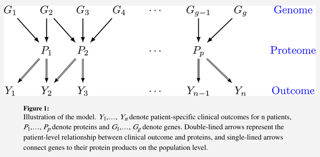
- clinical outcomes $Y={Y_1,\ldots,Y_n}$ for $n$ patients
- proteins $P={P_1,\ldots,P_p}$
- genes $G={G_1,\ldots,G_g}$
The genomic information is incorporated through modifying the downstream effects of a selective subset of proteins on clinical outcomes. The significance of these effects is identified by a novel subject-specific variable selection technique, which allows for the detection of protein markers on the patient level.
- an example: a protein BCL2 is found to be prognostic only for a subgroup of patients with concordant homogeneous genomic features, which may guide certain targeted BCL2-antagonists.
- such “genomically homogeneous” patients may have favorable (or unfavorable) responses to a certain treatment which is perhaps not as effective or dominant for other heterogeneous subgroups.
Aim: build models that help to improve the understanding of the biological underpinnings of prognostic pro-teogenomic biomarkers on the patient level; - and perhaps provide a new insight into tumor heterogeneity that potentially leads to the development of novel personalized treatments.
Data description
The Cancer Genome Atlas (TCGA): a project that was launched in 2005 to explore, evaluate and characterize the genomic and proteomic landscape of over 30 human cancers, both common and rare forms.
- use RNA-seq, a next-generation sequencing technology, to generate genomic data at a fine molecular resolution
- RNA-seq has very low background noise and is very accurate in measuring gene expression levels compared to traditional technologies such as microarrays
gene expression: since May 2012, the pipeline RNASeqV2 has been adopted by TCGA to generate the Level 3 expression data: use MapSlice to align the sequence data and RSEM to quantify transcript abundances
proteomic data: the proteomic data on the same tumor samples have been generated at UT MD Anderson Cancer Center using RPPAs, a high-throughput antibody-based technique.
clinical information: cancer stage, histologic subtype, and survival times, with some cancers having more mature survival data with a sufficient number of events and follow-up times to allow us to build prognostic models for those cancers.
The paper focuses on integrating genomic, proteomic and clinical information to select relevant prognostic markers
- detect patient-level prognostic protein markers
- investigate the mechanism of genomically driven protein markers
Overview of the model
One naive way is to regress clinical outcomes on the genomic and proteomic data and apply a variable selection technique to select protein markers.
- But it does not consider interactions between genes and proteins.
- One remedy is to add interaction terms into the model, but the biochemistry of the interaction is often quite complex
To allow for flexible interactions, one can incorporate varying coefficients into the regression model.
But that cannot account for tumor heterogeneity because the selected biomarkers are presumably the same for all patients.
Three major innovations:
- sparsity in both protein-outcome and protein-gene relationships.
- sparsity in the protein-outcome relationship
- sparsity in the protein-gene relationship
- accounting for genomic heterogeneity
- functional nonlinearity in protein-gene relationships
Bayesian hierarchical varying-sparsity regression model
- $Y_i$: survival time
- $P_i = (P_{i1},\ldots, P_{ip})$: protein expressions
- for each $P_{ij}$, gene expression $G_{ij}=(G_{ij1},\ldots, G_{ijq_j})$
expect that
- some of the proteins may not be relevant to every patient’s outcome
- the effect $\beta_j$ of each protein may also vary across patients
Propose a varying-coefficient model that allows $\beta_j$ to vary with $G_{ij}$ in terms of both strength and sparsity,
\[\sum_{j=1}^pP_{ij}\beta_j(G_{ij})\]Model varying-sparsity coefficient and protein selection
two motivations for $\beta_j(G_{ij})$ as a smooth function
- reflect the assumption that patients with similar genomic characteristics should have similar protein markers, and ensure the sparsity of $\beta_j$ changes smoothly with the genes $G_{ij}$
- a way of continuously “borrowing strength” by pooling genomic information from “neighboring” patients
construct $\beta_j$ as the sum of the spline functions
\[\beta_j(G_{ij}) =\sum_{k=1}^{q_j}f_{jk}(G_{ijk})\]take a hard-thresholding operator
\[\beta_j(G_{ij}) = h\left\{\sum_{k=1}^{q_j}f_{jk}(G_{ijk}), \lambda_j\right\}\]VCM can be viewed as a special case by fixing $\lambda_j=0$.
Hierarchical varying-sparsity accelerated failure time model
Propose to embed accelerated failure time (AFT) in BEHAVIOR framework,
\[Y_i = \log(T_i) = \mu+\sum_{j=1}^pP_{ij}\beta_j(G_{ij}) +\sigma\varepsilon_i\]Survival times are often observed subject to censoring.
- $C_i$: independent censoring time
instead of directly observing the survival time $T_i$, we observe $T_i^\star = \min(T_i, C_i)$ and $\Delta_i = I(T_i < C_i)$.
Let
\[W_i = \frac{\log(T_I^\star) - \sum_{j=1}^pP_{ij}\beta_j}{\sigma}\]then the likelihood is given by
\[L(\beta,\sigma\mid \text{Data}) = \prod_{i=1}^n f(W_i)^{\Delta_i} S(W_i)^{1-\Delta_i}\]where $f(\cdot)$ and $S(\cdot)$ are the respective density and survival functions of $\varepsilon_i$.
Prior and gene selection
Spline coefficients
choose a large enough number of knots to capture the local features and regularize the spline coefficients by imposing an improper Gaussian random walk prior
\[\sum_{k=1}^{q_j}f_{jk}(G_{ijk}) = \sum_{k=1}^{q_j}G_{ijk}^\star\alpha_{jk}^\star +\sum_{k=1}^{q_j}G_{ijk}\alpha_{jk}^0+\alpha_j\]impose a parameter-expanded normal-mixture-of-inverse-gamma (peNMIG) prior on each of $\alpha_j, \alpha_{jk}^0$ and $\alpha_{jk^\star}$. Take $\alpha_{jk}^\star$ as an example,
Multiplicatively expand $\alpha_{jk}^\star = \eta_{jk}\xi_{jk}$, where
- $\eta_{jk}$ is a scalar parameter indicating the relevance of $\alpha_{jk}^\star$
- $\xi_{jk}$ is a vector of the same size as $\alpha_{jk}^\star$.
Prior for gene selection
assign a spike-and-slab prior on $\eta_{jk}$
\[\eta_{jk}\sim \gamma_{jk}N(0, \tau_{jk}) + (1-\gamma_{jk})N(0, \nu_0\tau_{jk})\]where $\gamma_{jk}\sim Bern(p)$ and $\nu_0$ is a fixed very small number.
for each element of vector $\xi_{jk} = (\xi_{jk}^{(i)})$, impose a normal mixture prior $0.5N(1, 1) + 0.5N(-1,1)$ which avoids assigning too much mass around zero and hence discourage small effects
Prior for protein selection
a non-informative prior $\lambda \sim Unif(0, b\lambda)$.
Assume a conjugate prior for the variance parameter $\sigma^2\sim IG(a_\sigma, b_\sigma)$.
Posterior Inference and Prediction
sample via MCMC algorithm
suppose we have a new patient with protein and gene expressions $(P_{n+1}, G_{n+1})$ and want to predict the survival time.
transform $\alpha_j, \alpha_{jk}^0, \alpha_{jk}^\star$ back to ${\alpha_{jk}}_{k=1}^{q_j}$, then
\[E[\log(T_{n+1}\mid \text{Data})] \approx \frac 1L \sum_{l=1}^L\sum_{j=1}^p P_{n+1, j}\beta_j^{(l)}(G_{n+1,j})\]Simulations
- generate $p = 9$ proteins as $P_{ij}\sim N(0, 1)$
- for each protein $j$, generate $G_{ij}=(G_{ij1},\ldots, G_{ijq_j})\sim N(0, I_{q_j})$, where $q_1=q_2=2, q_3=q_4=3, q_5=\cdots=q_9=1$.
- use the first three proteins to generate survival times
with $\sigma=1, n=400$, and $\beta_j(G_{ij})=h(\theta_j(G_{ij}),\lambda)$, where $\theta_1(G_{i1}) = -2G_{i11}, \theta_2(G_{i2})=G_{i21}^2-1$ and $\theta_3(G_{i3})=2\sin(\pi G_{i31}/2)$/
-
error term $\epsilon_i$ is simulated from a standard extreme value distribution $f(\epsilon_i) = \exp(\epsilon_i)\exp(-\exp(\epsilon_i))$.
- sample censoring time such that the censoring rate is close to that of the KIRC data
- generate independent test dataset in the same manner
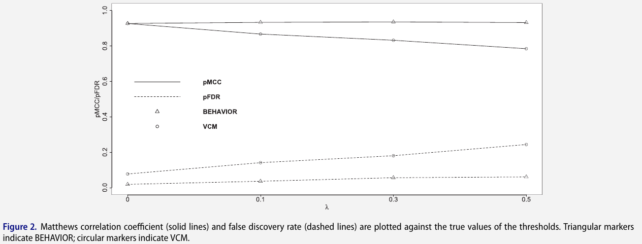
- consider four scenarios with different true thresholds
to assess the two-level variable selection performance, calculate true positive rate, FDR, Matthews correlation coefficient (MCC) and area under the receiver operating characteristic curve (AUC)
Pan-Cancer Proteogenomic Analyses
- focus on 12 core signaling pathways that have known/established role in cancer progression and development
- retrieve and match genomic, proteomic and clinical data using software TCGA-Assembler and map them to the 12 pathways
- consider four cancers for which TCGA has the most mature survival data
- apply BEHAVIOR separately to each type of cancer and pathway combination (4x12=48 analyses)
- run four parallel MCMC chains, each with 500,000 iterations, a burn-in of 250,000 iterations and a thinning of 5
Pan-Cancer Analysis
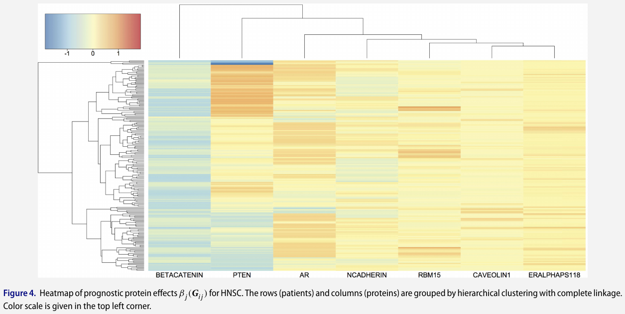
Protein-based analysis
some protein markers are shared by multiple cancers while others are exclusively relevant to one cancer
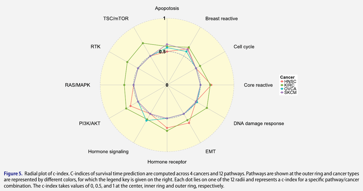
Pathway-based analysis
C-index measures how well the survival model predicts the data and is defined as the ratio of the number of concordant predicted survival times against the number of all possible pairs that can be ordered,
\[C-\text{index} = \frac {1}{\vert O\vert} = \sum_{(i,j)\in O}I(\hat T_i < \hat T_j)\]where $O={(i, j)\mid \Delta_i=1, Y_i < Y_j}$
Detailed Analysis for Kidney Renal Clear Cell Carcinoma
- 428 patients, 286 of whom are censored (67% censoring rate)
- median survival time is 2256 days from Kaplan-Meier estimates
Discussion
- currently only considers one cancer at a time and therefore may be less efficient that a joint approach that models different cancers simultaneously
- only use transcript expressions of known isoforms that are available from TCGA. Inference on novel isoforms is by itself an interesting research topic.
- it does not take into account the uncertainty or error in the data quantification and bioinformatics pre-processing procedures for the raw-level transcriptomic and proteomic data
- although the paper focus on prognostic models, a varying sparsity coefficient can be incorporated into many other models.
The code is available at https://github.com/jasa-acs/Bayesian-Hierarchical-Varying-sparsity-Regression-Models-with-Application-to-Cancer-Proteogenomics, but the source code is hidden, only the executable program.