Fitting to Future Observations

Posted on Jul 21, 2022

This note is for Jiang, Y., & Liu, C. (2022). Estimation of Over-parameterized Models via Fitting to Future Observations (arXiv:2206.01824). arXiv.

sample $S={(x_i, y_i):i=1,\ldots,n}$ of measurements $(x, y)$ on each of $n$ items from a population $\bbP$ is modeled by

with unknown parameter $\theta\in \IR^p$.

Also write

where the distribution of $X$ is assumed to be independent of $\theta$

• $\ell(\theta\mid x, y)$: log-likelihood function of $\theta$, based on the model $\bbP_\theta^{(n)}$
• loss function: $L(\theta\mid x, y) = -\ell(\theta\mid x, y)$

Define the best model as $\bbP_{x,\theta}^{(n)}$ that minimizes the expected loss with respect to the population, that is, $\bbP_{x,\theta}$ with some $\theta$ in

A modelling strategy is said to be valid iff \(\lim_{n\rightarrow\infty}\bbP_\theta^{(n)}=\bbP\) weakly for any $\theta\in \Theta_\star^{(n)}$ and some distance measure for probability distributions $\delta(\cdot,\cdot)$.

Consider two models $\bbP_{1,\theta}^{(n)}, \theta\in \Theta\subset \IR^{p_1}$, and $\bbP_{2,\xi}^{(n)}, \xi\in \Xi\subset \IR^{p_2}$, with bounded likelihood functions for a fixed sample size $n$ and some distance measure $\delta(\cdot,\cdot)$. Model 1 is said to be more efficient than Model 2 iff $E_{(X, Y)}\delta(\bbP_{1,\theta}^{(n)},\bbP)\le E_{X,Y}\delta(\bbP_{2,\xi}^{(n)},\bbP)$ for any $\theta \in \Theta_\star=\left\{\theta:E_{(X,Y)\sim \bbP}[L_1(\theta\mid X, Y)]=\min_{\tilde \theta}E_{(X,Y)\sim \bbP}[L_1(\tilde \theta\mid X, Y)]\right\}$ and $\xi \in \Xi_\star=\left\{\xi:E_{(X,Y)\sim \bbP}[L_2(\xi\mid X, Y)]=\min_{\tilde\xi}E_{(X,Y)\sim \bbP}[L_2(\tilde \xi\mid X, Y)]\right\}$, where $L_1$ and $L_2$ are the loss functions of model $\bbP_{1,\theta}^{(n)}$ and $\bbP_{2,\xi}^{(n)}$, respectively.

Different from Box’s “All models are wrong but some are useful”, the paper said “models, as simple-but-not-simpler approximations to $\bbP$, depend on the observed data and often change as more data are available.”

The definition of efficiency emphasises on the importance of modeling for future observations and suggests in auto-modeling with over-parameterized models, an imputation method be used to approximate the population.

An Imputation and Estimation Algorithm

Find an approximate solution to the desired optimization problem

by optimizing its sample counterpart, with a preference for simple models to control the deviation of the estimate of $\theta$,

where $\hat\bbP$ is the empirical distribution defined by the sample ${(x_i, y_i):i=1,\ldots,n}$.

Take a type of generalized $L_1$ penalty,

Write the target objective function,

where

$G_{\hat \bbP}(\theta, \lambda)$ is minimized over $\theta$ at $\theta = \hat\theta$ for given $\lambda$, the remaining term $V_{\bbP,\hat\bbP}(\theta,\lambda)$ serves as a measure of validation.

Desire to choose $\lambda$ to minimize $E_{(X, Y)\sim \bbP}[L(\theta\mid X, Y)]$, then looks for a solution to have

for all $i=1,\ldots, p$.

Consider a weaker alternative condition: $V_{\bbP,\hat\bbP}(\theta,\lambda)$ is required to be approximately a constant in a neighborhood of $\hat \theta$. (why?)

for all $i=1,\ldots,p$.

is $\hat \lambda_i$ a function of $\theta_i$?

Create one future observation $(x, y)$

1. take a bootstrap sample ${(\tilde x_i, \tilde y_i):i=1,\ldots, n}$. Denote by $\tilde \bbP$ the corresponding empirical distribution.
2. find the bootstrap estimate $\tilde\theta$, that is, $\tilde\theta$ is obtained by minimizing $G_{\hat \bbP}(\theta,\lambda)$ over $\theta$ subject to

1. draw $x$ from ${x_i:i=1,\ldots,n}$ at random and simulate $y$ from the fitted predictive model

Numerical Optimization Methods

Find a pair of solutions $\hat\theta$ and $\hat\lambda$ that minimize both $G_{\hat \bbP}(\theta,\lambda)$ and $V_{\bbP,\hat\bbP}(\theta,\lambda)$, as functions of $\theta$ (???), at $\theta=\hat\theta$ for some $\lambda=\hat\lambda$.

Method of Lagrange multipliers

subject to the system of constraints $\partial G_{\hat\bbP}(\theta,\lambda)/\partial\theta=0$. The Lagrange function of $(\theta,\lambda,\phi)$ to be minimized becomes

Coordinate Descent Algorithm

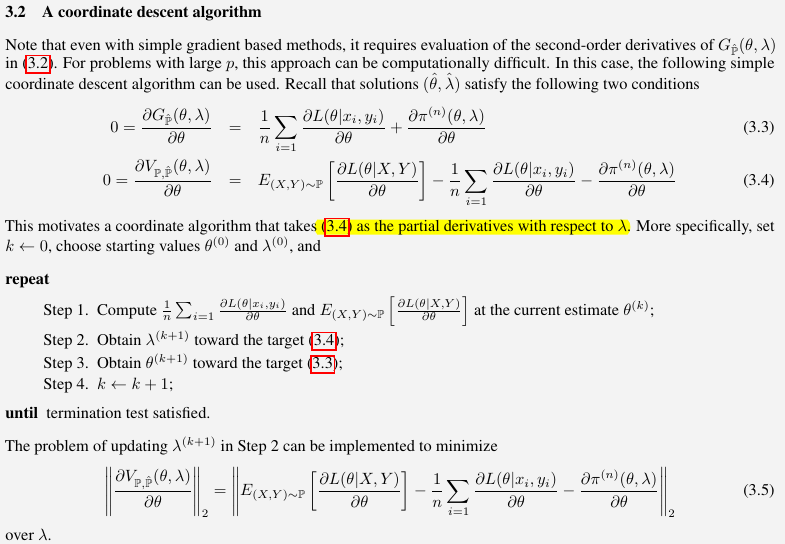
• Take another perspective of (3.3), it is just to minimize $G_{\hat\bbP}(\theta, \lambda)$. Thus, we can directly take advantage with existing nonlinear programming solvers, such as Ipopt (Interior Point Optimizer).
• For (3.4) and (3.5), since $\theta_2,\cdots,\theta_m\ge 0$, then

and hence

Application: Many-Normal-Means

Make inference on the unknown means $\mu_1,\ldots, \mu_n$ from the sample $Y_1,\ldots, Y_n$ with the model $Y_i\mid {\mu_1,\ldots,\mu_n}\sim N(\mu_i,1),i=1,\ldots,n$, where $Y_1,\ldots,Y_n$ are independent of each other.

Re-formulate the problem: $Y_1,\ldots,Y_n$ is assumed to be a sample from a single population and view $\mu_1,\ldots,\mu_n$ as missing values taken from some unknown population. That is,

Take a simple discrete distribution at $m\ge n$ unknown points $\eta_1\le \eta_2\le\cdots\le \eta_m$ with the probability mass $\Pr(\mu = \eta_k) = \alpha_k, k=1,\ldots,m$. Then the observed-data likelihood based on $Y_i$ is given by $1/{\sqrt{2\pi}}\sum_{k=1}^m\alpha_k\exp(-\frac{(Y_i-\eta_k)^2}{2})$

Auto-modeling framework is used for fitting the discrete distribution model $\bbP_\theta^{(n)}$, which provides an approximation to the true distribution.

For simplicity-preference function, write $\theta_1=\eta_1, \theta_k=\eta_k-\eta_{k-1}$ for $k=2,\ldots,m$ and $\theta_{m+k}=\alpha_k$ for $k=1,\ldots,m$. Take the $L_1$ penalty on $(\theta_2,\ldots,\theta_m)’\in \IR^{m-1}$, that is $\pi_\lambda^{(n)}(\theta) = \sum_{k=2}^m\lambda_k\vert \theta_k\vert$, where $\lambda_k\ge 0$ and $k=2,\ldots, m$.

then

Alternatively, we can use finite difference to approximate the derivatives, such as the JuliaDiff/FiniteDifferences.jl package in Julia, but attention that forward_fdm might be needed due to singularity issue of log function.

• MLE: $\hat\mu^{MLE}_i=y_i$.

• James-Stein Estimator:

which shrinks the MLE of each $\mu$ towards the overall sample mean of the observed data.

• g-modeling: According to Narasimhan and Efron (2020), Empirical Bayes inference assumes an unknown prior density $g(\theta)$ has yield (unobservable) $\Theta_1,\ldots,\Theta_N$, and each $\Theta_i$ produces an independent observation $X_i$ from $p_i(X_i\mid \Theta_i)$. The marginal density $f_i(X_i)$ is a convolution of the prior $g$ and $p_i$. The Bayes deconvolution problem is to recover $g$ from the data. Generally, the estimation of $g$, so-called g-modeling, is difficult, but Narasimhan and Efron (2020) proposed to restrict the prior $g$ to lie within a parametric family of distributions and claimed that the results are more encouraging. Their R package deconvolveR is available on CRAN.

For the many normal means example, just call

result <- deconv(tau = tau, X = x, deltaAt = 0, family = "Normal")

where x is the observed data, and tau is a vector of discrete support points for $\theta$.

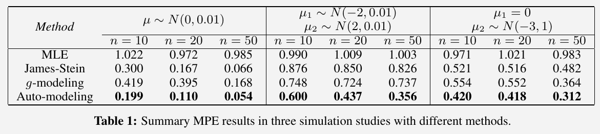
For simplicity, I skip the step of approximation of $\bbP$ by bootstrap samples, and instead directly use the true $\bbP$. My results are as follows,

julia> @time many_normal_means(n=10,K=200,case=1)
409.362780 seconds (3.79 G allocations: 408.156 GiB, 13.74% gc time)
1×4 Matrix{Float64}:
 0.951092  0.297215  0.18758  0.174413

julia> @time many_normal_means(n=10,K=200,case=2)
1166.330146 seconds (10.30 G allocations: 1.085 TiB, 14.45% gc time)
1×4 Matrix{Float64}:
 1.05033  0.948022  0.849796  0.684122

julia> @time many_normal_means(n=10,K=200,case=3)
873.212648 seconds (7.60 G allocations: 818.290 GiB, 14.50% gc time, 1.37% compilation time)    
1×4 Matrix{Float64}:
 1.01645  0.565332  0.428163  0.438326

julia> @time many_normal_means(n=20,K=200,case=1)
1506.267866 seconds (11.68 G allocations: 1.780 TiB, 14.42% gc time)
1×4 Matrix{Float64}:
 1.0176  0.151387  0.0856947  0.107758

julia> @time many_normal_means(n=20,K=200,case=2)
5058.591486 seconds (38.67 G allocations: 5.893 TiB, 13.97% gc time, 0.00% compilation time)
1×4 Matrix{Float64}:
 0.994893  0.85625  0.764716  0.488117

julia> @time many_normal_means(n=20,K=200, case=3)
4469.796364 seconds (32.48 G allocations: 4.950 TiB, 14.42% gc time)
1×4 Matrix{Float64}:
 1.05389  0.511735  0.323881  0.460926

We observe that

• Except the results of g-modeling, others are close to the reported results in the paper.
• Sometimes g-modeling can outperform auto-modeling, but I did not deliberately select its parameters. The paper also did not discuss how they choose the parameters for this method.
• Currently the program is quite slow, and the computational burden is mainly Step 3 in the coordinate descent algorithm. Is there any speed-up strategies?

References

• Narasimhan, B., & Efron, B. (2020). deconvolveR: A G-Modeling Program for Deconvolution and Empirical Bayes Estimation. Journal of Statistical Software, 94, 1–20.