Neuronized Priors for Bayesian Sparse Linear Regression
Posted on
This note is for Shin, M., & Liu, J. S. (2021). Neuronized Priors for Bayesian Sparse Linear Regression. Journal of the American Statistical Association, 1–16.
Practically, the routine use of Bayesian variable selection methods has not caught up with the non-Bayesian counterparts such as Lasso, likely due to difficulties in both computations and flexibilities of prior choices.
The paper propose the neuronized priors to unify and extend some popular shrinkage priors, such as Laplace, Cauchy, horseshoe, and spike-and-slab priors.
A neuronized prior can be written as the product of a Gaussian weight variable and a scale variable transformed from Gaussian via an activation function.
Compared with classic spike-and-slab priors, the neuronized priors achieve the same explicit variable selection without employing any latent indicator variables.
Consider standard linear regression model,
\[y=X\theta+\epsilon\]To model the sparsity of $\theta$ when $p$ is large, a popular choice is the one-group continuous shrinkage prior, which can be represented as a hierarchical scale-mixture of Gaussian distributions.
\[\theta_j\mid \nu_w^2,\tau_j^2 \sim N(0, \nu_w^2\tau_j^2)\\ \tau_j^2\sim \pi_\tau, \nu_w\sim \pi_g\]where
- the local shrinkage parameter $\tau_j^2$ governs the shrinkage level of an individual parameter
- the global shrinkage parameter $\nu_w^2$ controls the overall shrinkage effect
Choice of $\pi_\tau$:
- the Strawderman-Berger prior: a mixture of gamma distributions
- Bayesian Lasso: an exponential distribution
- horseshoe prior: a half-Cauchy distribution
- generalized double Pareto: a mixture of Laplace distributions
- Dirichlet-Laplace prior: the product of a Dirichlet and a Laplace random variable
Another popular class of shrinkage prior: spike-and-slab (SpSL), also known as two-group mixture priors
\[\theta_j\mid \gamma_j\sim (1-\gamma_j)\pi_0(\theta_j) + \gamma_j\pi_1(\theta_j)\\ \gamma_j\sim Bernoulli(\eta)\]where
- $\pi_0$ is the spike, typically chosen to be highly concentrated around zero
- $\pi_1$ is the slab, relatively disperse
discrete vs continuous SpSL
- discrete SpSL: a point-mass at zero is used for $\pi_0$
- continuous SpSL: a continuous SpSL. Common choices are Gaussian distributions with a small and a large variance.
For a nondecreasing activation function $T$ and hyper-parameters $\alpha_0$ and $\tau_w$, a neuronized prior for $\theta_j$ is defined as \(\theta_j:=T(\alpha_j-\alpha_0)w_j\) where $\alpha_j\sim N(0, 1)$ and the weight $w_j\sim N(0, \tau_w^2)$, all independently for $j=1,\ldots,p$.
It shows that for most existing shrinkage priors, one can find specific activation activation functions such that the resulting neuronized priors approximate the existing ones.
Advantages:
- unification
- Flexibility and efficient computation
- Desirable theoretical properties
Neuronization of Standard Sparse Priors
Discrete and Continuous SpSL
- if $T(t)=\max(0, t)$ is the ReLU function, the resulting prior is identical to SpSL priors
when $\alpha_0 = 0$, $T(\alpha_j - \alpha_0)$ follows an equal mixture of the point-mass at zero and the half standard Gaussian. It implies that the marginal density of $T(\alpha_j)w_j$ is a SpSL distribution of the form
\[\begin{align} \theta \mid \gamma \sim (1-\gamma) \delta_0(\theta) + \gamma \pi(\theta)\\ \gamma \sim Bernoulli(1/2)\,, \end{align}\]where $\pi$ is the marginal density of the product of two independent standard Gaussians, which is shown to have an exponential tail.
continuous SpSL priors can be obtained by adopting a leaky ReLU activity function, $T(t) = \max{ct, t}$ for some $c < 1$.
Generally, $\alpha_0$ controls the prior probability of sparsity:
\[P(T(\alpha_j - \alpha_0) = 0\mid \alpha_0) = P(\alpha_j < \alpha_0 \mid \alpha_0) = \Phi(\alpha_0)\]Then for $\eta \in (0, 1)$, choose $\alpha_0 = -\Phi^{-1}(\eta)$ to achieve the desired sparsity.
For the sparsity parameter $\eta$, someone takes the Beta hyper-prior $\eta\sim Beta(a_0, b_0)$.
The neuronized priors can acommodate this Bernoulli-beta hyper-prior by adopting a hyper-prior on $\alpha_0$
Bayesian Lasso
- $T(t)=t$ approximates the Bayesian Lasso
the Laplace density differs from the neuronized prior only by a term $z^{-1}$ in the integrand
the tail of this neuronized prior decays at an exponential rate like the Bayesian Lasso prior
Horseshoe, Cauchy and Their Generalizations
any polynomial tails of the local shrinkage prior can be constructed by neuronizing a Normal random variable through an exponential function, up to a logarithmic factor.
consider the following class of activating functions
\[T(t) = \exp(\lambda_1\sign(t)t^2 + \lambda_2 t + \lambda_3)\]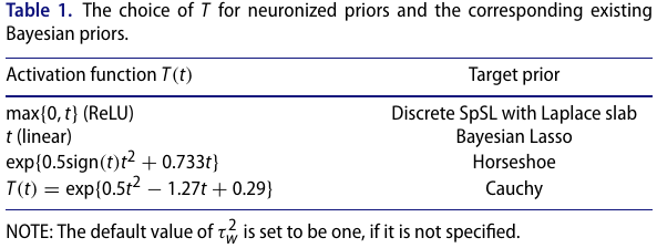
Managing Neuronized Priors
Find the Activation function to match a given prior
To find an activation function $T$ so that the resulting neuronized prior matches a desired target distribution $\pi(\theta)$.
define a class of activation functions parameterized by ${\lambda_1,\phi}$
\[T(t) = \exp(\lambda_1\sign(t)t^2) + B(t)\phi\]Once $\lambda_1$ is fixed, generate a large number $S$ of iid samples from the neuronized priors: $\tilde\theta_i$, and also generate $\theta_i\sim \pi(\theta)$. Then minimize the discrepancy by using a grid search or a simulated annealing algorithm.