Empirical Bayes
Posted on
This note is based on Sec. 4.6 of Lehmann, E. L., & Casella, G. (1998). Theory of point estimation (2nd ed). Springer.
\[\def\bx{\mathbf{x}}\]Empirical Bayes is generalization of single-prior Bayes estimation, and it falls outside of the formal Bayesian paradigm.
EB estimators tend to be more robust against misspecification of the prior distribution.
Consider the model
\[X_i\mid \theta \sim f(x\mid \theta), i=1,\ldots,p;\quad \Theta\mid \gamma\sim \pi(\theta\mid \gamma)\,,\]but we now treat $\gamma$ as an unknown parameter of the model, which also needs to be estimated.
Calculate the marginal distribution of $\bX$, with density
\[m(\bx\mid \gamma) = \int \prod f(x_i\mid \theta)\pi(\theta\mid\gamma)d\theta\,.\]It is most common to take $\hat\gamma(\bx)$ to be the MLE of $\gamma$, but this is not essential.
Substitute $\hat\gamma(\bx)$ for $\gamma$ in $\pi(\theta\mid \gamma)$ and determine the estimator that minimizes the empirical posterior loss
\[\int L(\theta,\delta(\bx))\pi(\theta\mid \bx,\hat\gamma(\bx))d\theta\,,\]and this minimizing estimator is the empirical Bayes estimator.
Example: Normal Empirical Bayes
\[m(\bx\mid \tau^2) =\int \prod_{i=1}^nf(x_i\mid \theta)\pi(\theta\mid \tau^2)d\theta = \frac{1}{(2\pi)^{n/2}}\frac{1}{\sigma^n}\left(\frac{\sigma^2}{\sigma^2+n\tau^2}\right)^{1/2}\exp\left(-\frac 12\left[\frac{\sum(x_i-\bar x)^2}{\sigma^2}+\frac{n\bar x^2}{\sigma^2+n\tau^2}\right]\right)\]The MLE of $\sigma^2 + n\tau^2$ is given by $\max{\sigma^2,n\bar x^2}$, and substitute into the single-prior Bayes estimator, we obtain the EB estimator
\[E(\Theta\mid \bar x,\hat\tau) = \left(1-\frac{\sigma^2}{\max(\sigma^2, n\bar x^2)}\right)\bar x\,.\]We can still consider $\pi(\theta\mid x,\hat\gamma(x))$ to be a “legitimate” posterior density, but the prior distribution that leads to such a posterior may sometimes not be proper.
Example: Empirical Bayes Binomial
Consider
\[X_k \sim Binomial(p_k, n), \qquad p_k\sim Beta(a, b), k=1,\ldots,K\]The single-prior Bayes estimator of $p_k$ under squared error loss is
\[\delta^\pi(x_k) = E(p_k\mid x_k,a,b) = \frac{a+x_k}{a+b+n}\,.\]In the EB model, consider these hyperparameters unknown and estimate them. The marginal distribution is
\[m(\bx\mid a, b) = \prod_{k=1}^K\binom{n}{x_k}\frac{\Gamma(a+b)\Gamma(a+x_k)\Gamma(n-x_k+b)}{\Gamma(a)\Gamma(b)\Gamma(a+b+n)}\]The MLEs $\hat a, \hat b$ are not expressible in closed form, but we can calculate them numerically and construct the EB estimator
\[\delta^{\hat\pi}(x_k)=\frac{\hat a+x_k}{\hat a+\hat b+n}\,.\]The Bayes risk performance of the EB estimator is often “robust”; that is, its Bayes risk is reasonably close to that of the Bayes estimator no matter what values the hyperparameters attain.
For the situation of Corollary 3.3,
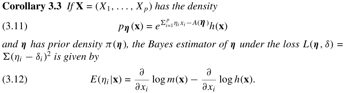
with prior distribution $\pi(\eta\mid \lambda)$, suppose $\hat \lambda(x)$ is the MLE of $\lambda$ based on $m(\bx\mid \lambda)$. Then, the empirical Bayes estimator is
\[E(\eta_i\mid \bx,\hat\lambda) = \frac{\partial}{\partial x_i}m(\bx\mid \hat(\bx)) - \frac{\partial}{\partial x_i}\log h(\bx)\,.\]