Conformal Inference

Posted on Sep 22, 2021 (Update: Sep 22, 2022) 0 Comments

Tags: Conformal Inference

The note is based on Lei, J., G’Sell, M., Rinaldo, A., Tibshirani, R. J., & Wasserman, L. (2018). Distribution-Free Predictive Inference for Regression. Journal of the American Statistical Association, 113(523), 1094–1111. and Tibshirani, R. J., Candès, E. J., Barber, R. F., & Ramdas, A. (2019). Conformal Prediction Under Covariate Shift. Proceedings of the 33rd International Conference on Neural Information Processing Systems, 2530–2540.

Let $U_1,\ldots, U_n$ be i.i.d. (or weaker assumption of exchangeability) samples of a scalar random variable. For a given miscoverage level $\alpha\in (0,1)$, and another i.i.d. sample $U_{n+1}$,

• if $\lceil (n+1)(1-\alpha)\rceil \le n$, by exchangeability, the rank of $U_{n+1}$ is uniformly distributed over the set ${1,\ldots, n+1}$

\[P(U_{n+1}\le U_{(\lceil (n+1)(1-\alpha)\rceil)}) = \frac{\lceil (n+1)(1-\alpha)\rceil}{n+1} \ge 1-\alpha\]

• otherwise

\[P(U_{n+1}\le \infty) = 1\ge 1-\alpha\]

Then for the regression problem, apply the above results on

\[\vert \epsilon_i\vert = \vert Y_i - \hat \mu(X_i)\vert\]

then

\[P(\vert Y_{n+1}-\hat \mu(X_{n+1})\vert \le \vert \epsilon\vert_{(\lceil (n+1)(1-\alpha)\rceil)}) \ge 1-\alpha\]

and then replace

\[\vert \epsilon\vert_{(\lceil (n+1)(1-\alpha)\rceil)}\]

with

\[\hat F_n^{-1}(1-\alpha)\]

Thus, we can form the prediction interval

\[C_{naive}(X_{n+1}) = \left[\hat\mu(X_{n+1})-\hat F_n^{-1}(1-\alpha), \hat\mu(X_{n+1})+\hat F_n^{-1}(1-\alpha)\right]\,.\]

Note that the above fitting does not involve the new point, the following improved strategy will incorporate the new point into the fitting procedure.

For each value $y\in \IR$ we construct an augmented regression estimator $\hat\mu_y$, which is trained on the augmented data set $(X_1, Y_1), \ldots, (X_n, Y_n), (X_{n+1}, y)$. Define

\[R_{y,i} = \vert Y_i-\hat\mu_y(X_i)\vert\,, i=1,\ldots,n\qquad R_{y,n+1}=\vert y-\hat \mu_y(X_{n+1})\vert\,,\]

and rank $R_{y,n+1}$ among the remaining fitted residuals $R_{y,1},\ldots, R_{y,n}$, just like the above $\vert \epsilon_i\vert$, then compute

\[\pi(y) = \frac{1}{n+1}\sum_{i=1}^{n+1}1\{R_{y,i}\le R_{y,n+1}\} = \frac{1}{n+1} + \frac{1}{n+1}\sum_{i=1}^n1\{R_{y,i}\le R_{y,n+1}\}\,.\]

the above one can be rewritten as \(\pi = \frac{1}{n+1}\sum_{i=1}^{n+1}1\{\vert \epsilon_{i}\vert \le \vert \epsilon_{n+1}\vert \}\,,\) which does not depend on $y$.

The constructed statistic $\pi(Y_{n+1})$ is uniformly distributed over the set ${1/(n+1),\ldots, 2/(n+1), \ldots, 1}$, then

\[P((n+1)\pi(Y_{n+1})\le \lceil (1-\alpha)(n+1)\rceil ) \ge 1-\alpha\,.\]

Then the conformal prediction interval at $X_{n+1}$ is

\[C_{conf}(X_{n+1}) = \left\{y\in \IR: (n+1)\pi(y) \le \lceil (1-\alpha)(n+1)\rceil\right\}\,.\]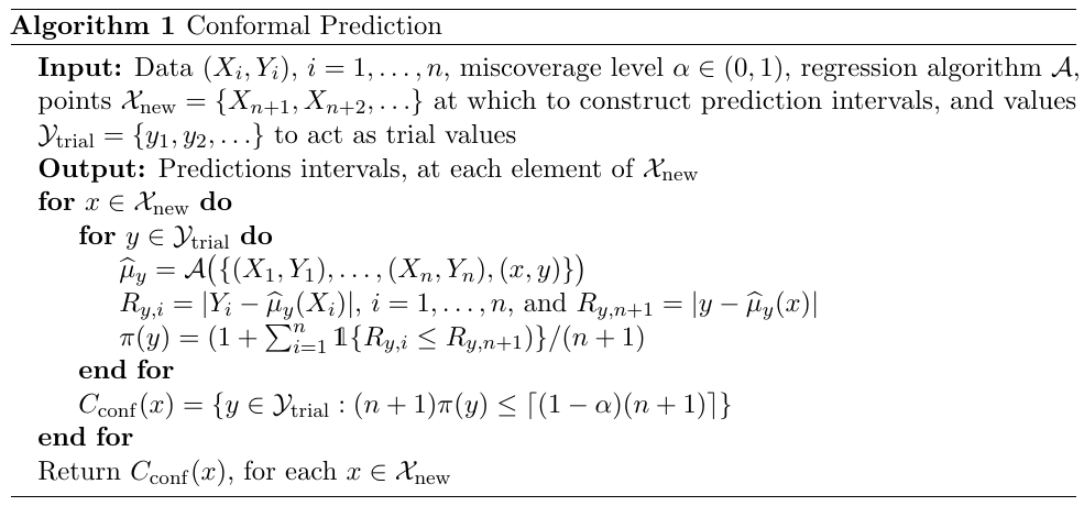

is the interval not necessarily continuous? If so, possible bisection method might help. This idea has been discussed in Ndiaye, E., & Takeuchi, I. (2021). Root-finding Approaches for Computing Conformal Prediction Set (arXiv:2104.06648).

but it is computationally intensive.

• In low-dimensional linear regression, the Sherman-Morrison updating scheme (TODO) can be used to reduce the complexity of the full conformal method, by saving on the cost of solving a full linear system each time the query point $(x, y)$ is changed.
• In high-dimensional regression, where we might use relatively sophisticated (nonlinear) estimators such as the lasso, performing efficient full conformal inference is still an open problem.

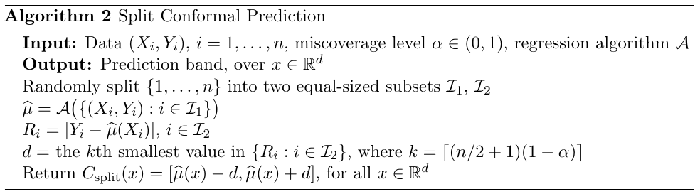
Alternatively, here is a cheap method separates the fitting and ranking steps using sample splitting,

Splitting improves dramatically on the speed of conformal inference, but introduces extra randomness into the procedure. One way to reduce this extra randomness is to combine inferences from several splits.

It sounds like $K$-fold cross-validation.

A balanced way is jackknife prediction.

It sounds like leave-one-out cross validation.

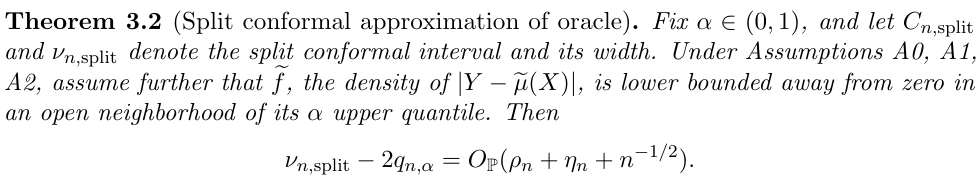
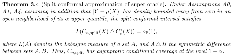
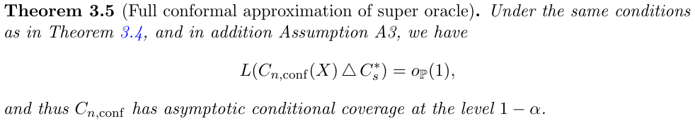
To quantify the accuracy of the prediction bands, compare their lengths to the length of the idealized prediction bands obtained by two oracles:

• super oracle: $C_s^\star(x) = [\mu(x)-q_\alpha, \mu(x) + q_\alpha]$
• regular oracle: $C_o^\star(x) = [\hat\mu_n(x)-q_{n,\alpha}, \hat\mu_n(x)+q_{n,\alpha}]$

The results are

• if the base estimator is consistent, then the two oracle bands have similar lengths

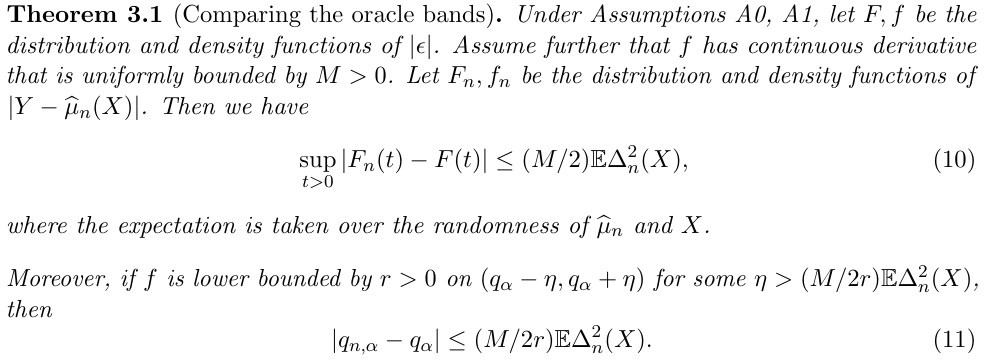
• if the base estimator is stable under resampling and small perturbations, then the conformal prediction bands are close to the oracle band

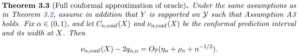
• if the base estimator is consistent, then the conformal prediction bands are close to the super oracle.

Conformal Prediction Under Covariate Shift

extend conformal prediction beyond the setting of exchangeable data, allowing for provably valid inference even when the training and test data are not drawn from the same distribution.

Denote $Z_i=(X_i, Y_i), i=1,\ldots,n$. Choose a score function $\cS((x, y), Z)$, a low value indicates that the point $(x,y)$ conforms to $Z$, and a high value indicates that $(x, y)$ is atypical relative to the points in $Z$. For example,

\[\cS((x, y), Z) = \vert y-\hat\mu(x)\vert\,.\]

What if multiple response? A $d$ ball might be appropriate.

Calculate the nonconformity scores

\[V_i^{(x, y)} = \cS(Z_i, Z_{1:n}\cup \{(x, y)\}), i=1,\ldots,n\]

and

\[V_{n+1}^{(x, y)} = \cS((x, y), Z_{1:n}\cup \{(x, y)\})\]

and include $y$ in the prediction interval $\hat C_n(x)$ if

\[V_{n+1}^{(x, y)} \le \mathrm{Quantile}(1-\alpha; V_{1:n}^{(x, y)}\cup \{\infty\})\]

The paper considers the setting where $(X_i, Y_i),i=1,\ldots,n+1$ are no longer exchangeable.

\[(X_i, Y_i) \sim_{i.i.d.} P = P_X \times P_{Y\mid X}, i=1,\ldots,n\\ (X_{n+1}, Y_{n+1}) \sim \tilde P = \tilde P_X \times P_{Y\mid X}, \,\text{independently}\,,\]

where the conditional distribution of $Y\mid X$ is assumed to be the same for both the training and test data. Such a setting is often called covariate shift.

Then instead of considering the empirical distribution

\[\frac{1}{n+1}\sum_{i=1}^n\delta_{V_i^{(x, y)}} + \frac{1}{n+1}\delta_\infty\,,\]

and we consider

\[\sum_{i=1}^n p_i^w(x)\delta_{V_i^{(x, y)}} + p_{n+1}^w(x)\delta_\infty\,,\]

where $w(X_i)=d\tilde P_X(X_i)/dP_X(X_i)$ and

\[p_i^w(x) = \frac{w(X_j)}{\sum_{j=1}^nw(X_j)+w(x)}, i=1,\ldots,n\quad p_{n+1}^w(x)=\frac{w(x)}{\sum_{j=1}^nw(X_j)+w(x)}\,.\]

Weighted Exchangeability

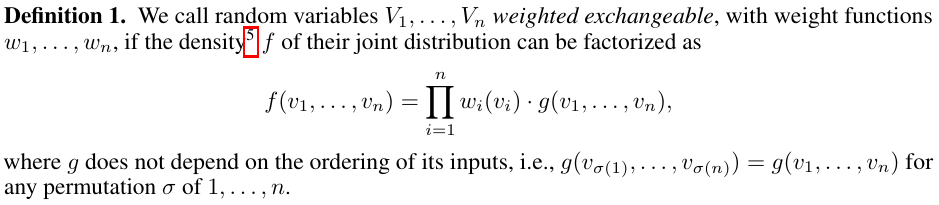
thus it can handle heterogeneous various? e.g., $x_i\sim N(\mu_i,\Sigma_i)$?