Generative Bootstrap/Multi-purpose Samplers

Posted on Sep 22, 2021 (Update: Oct 12, 2022)

This post is based on the first version of Shin, M., Wang, L., & Liu, J. S. (2020). Scalable Uncertainty Quantification via GenerativeBootstrap Sampler., which is lately updated as Shin, M., Wang, S., & Liu, J. S. (2022). Generative Multiple-purpose Sampler for Weighted M-estimation (arXiv:2006.00767; Version 2). arXiv.

Multiple Bootstrap Sampler [Shin et al. (2020)]

• construct a generator function of bootstrap evaluations, and it transforms the weights on the observed data points to the bootstrap evaluations
• it is implemented by one single optimization

A General Form of Bootstrap

Consider observations $y=\{y_1,\ldots, y_n\}$ generated from a true data-generating distribution $F_\theta$.

In many problems, a valid estimator of $\theta$ can be found as the solution of

the conventional bootstrap procedure for assessing statistical properties of the resulting estimator $\hat\theta$ relies on the generation of the bootstrap samples, $\hat\theta^{(b)},b=1,\ldots,B$, via the following competitions

where $w^{(b)} = \{w_1^{(b)},\ldots, w_n^{(b)}\}$ is independently generated from a distribution $H_w$.

some problems are not considering the parameters, for example, if we want to fit a spline and get the point-wise confidence interval at each point, i.e., obtaining the confidence interval bands. can this problem be treat in this framework?

• classic nonparametric bootstrap: $H_w=Multinomial(1/n,\ldots,1/n)$
• Bayesian bootstrap: the posterior distribution of the unknown sampling distribution under the Dirichlet process prior with its base measure converging to 0
• weighted likelihood bootstrap (WLB)

Generative Bootstrap Sampler

explicitly treat $\hat\theta_w$ as a function of $w$.

Once $\hat G$ is trained (how to train? what is the input and output?)

For $b=1,\ldots, B$

1. sample ${w_1^{(b)},\ldots, w_n^{(b)}}^T\sim H_w$
2. evaluate $\hat\theta^{(b)}=\hat G(w^{(b)})$

Generative Multi-purpose Sampler [Shin et al. (2022)]

Introduction

Consider observations $y=\{y_1,\ldots,y_n\}$, and the parameter of interest is denoted by $\theta\in\Theta\subset \IR^p$.

• predictors or covariate variables: $X = \{X_1,\ldots,X_n\}$, where each $X_i\in \IR^q$ for some $q$

A valid estimator of $\theta$ can be found for a large number of problems by solving the following (penalized) weighted M-estimation:

with

where

• $\ell_\eta$ is a suitable loss function chosen by the researcher
• $\eta\in\IR^+$ is an auxiliary parameter of the loss, and an example includes the quantile level $\eta\in (0, 1)$ in quantile regression models
• $u$ is a penalty function on the parameter with a tuning parameter $\lambda$ that can be set to zero for non-penalized settings.
• $w={w_1,\ldots,w_n}\in \cW$ is a vector of weights following distribution $\pi(\bfw)$

A simple example of this weighted M-estimation is bootstrapping Maximum Likelihood Estimators (MLEs);

The form applies to a wide range of statistical procedures, for example,

• classical bootstrap procedures can be expressed with $u(\theta)=0$, when the weight is the space of length-$n$ vectors of nonnegative integers and $w$ is repeatedly generated from Multinom($n;1/n,\ldots,1/n$). Then the resulting $\hat\theta_{w,\lambda}$’s correspond to the nonparametric bootstrap samples
• random weight bootstraps can be formulated by imposing a random distribution on $w$ that has a mean of one and a variance of one, and their theoretical properties, such as consistency of the bootstrap distribution towards the sampling distribution, were rigorously demonstrated in multiple articles.
  • a common practice of random weight bootstrap is to set $w\sim n\times \text{Dirichlet}(n;1,\ldots, 1)$ as in Bayesian Bootstrap and Weighted Likelihood Bootstrap
• Iterated bootstrap procedures, in which bootstrapped samples are iteratively bootstrapped, reduce the bias associated with a statistical inference procedure.
  • The double bootstrap procedures can be represented by setting a hierarchical weight distribution such that $s={s_1,\ldots,s_n}\sim \text{Multinomial}(n;1/n,\ldots,1/n)$ and $w\mid s\sim \text{Multinomial}(n;s_1/n,\ldots,s_n/n)$, and they can be used to correct the bias of a estimator, the coverage of a confidence interval, etc.
  • These iterated bootstraps provide more accurate corrections, referred to as second-order correctness or higher-order correctness, when compared to single bootstraps or asymptotic approximations

Iterative bootstrap for correcting the bias based on Martin, M. A. (1992). On the Double Bootstrap. In C. Page & R. LePage (Eds.), Computing Science and Statistics (pp. 73–78). Springer New York.

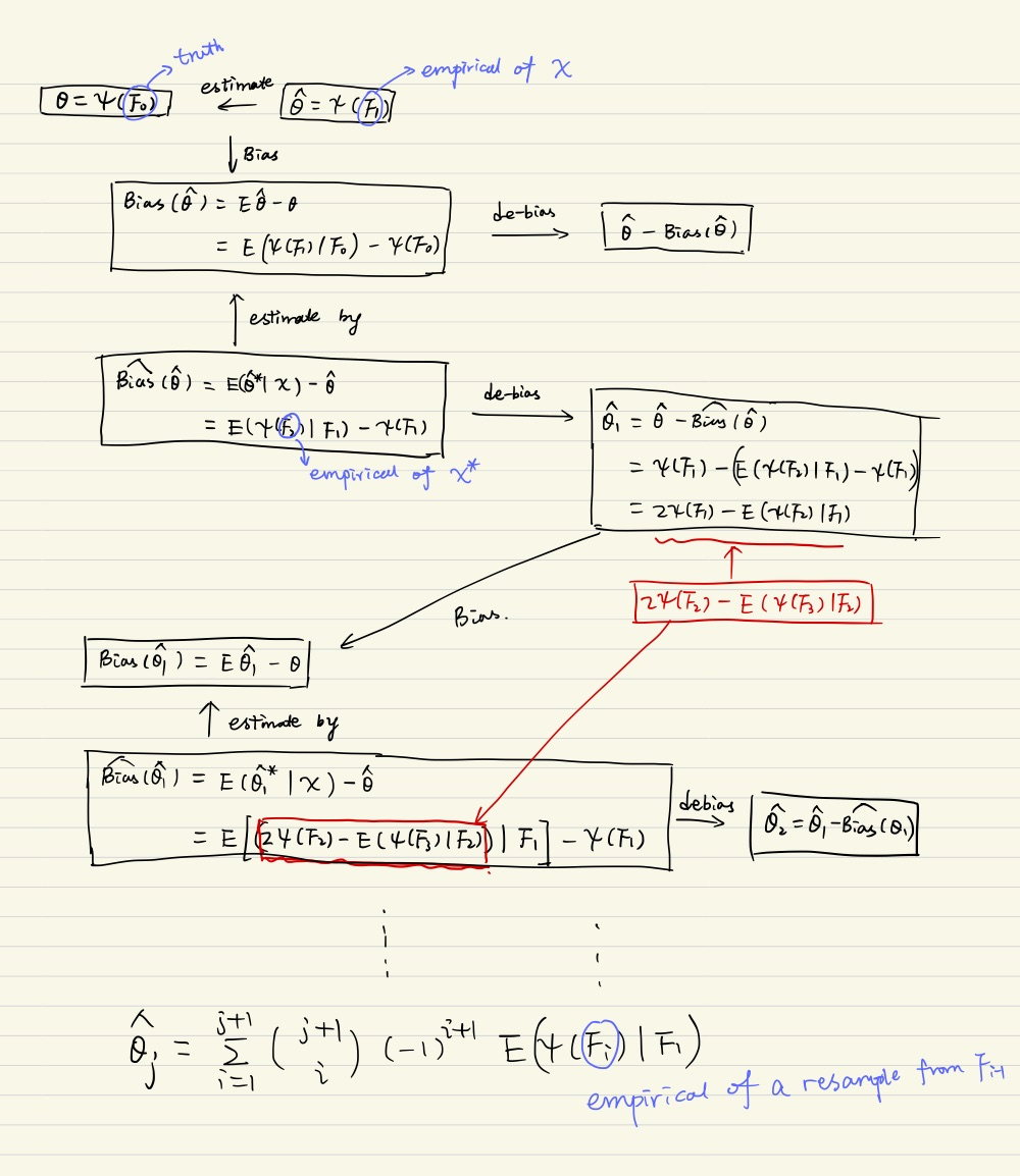
Let $I_1(\alpha, \cX)$ be a nominal $\alpha$-level confidence interval for the unknown parameter $\theta$. Denote the coverage probability by $\pi(\alpha) = P(\theta\in I_1(\alpha;\cX))$. The true coverage $\pi(\alpha)$ is often not exactly equal to the nominal coverage $1-\alpha$. The bootstrap estimate of $\pi(\alpha)$ is $\hat\pi(\alpha)=P(\hat\theta\in I_1(\alpha;\cX^\star)\mid \cX)$. To find $\beta_\alpha$ such that $\hat\pi(\gamma)=1-\alpha$.

\[\begin{align} \pi(\gamma) &= \frac 1B \sum_{b=1}^B1(\hat\theta\in \hat I_1(\gamma; \cX_b^\star)\mid \cX)\label{eq:I1}\\ &= \frac 1B \sum_{b=1}^B 1(p_b^\star > \gamma)\label{eq:pval} \end{align}\]

To calculate the interval in \eqref{eq:I1} for each bootstrap sample $\cX_b^\star$, perform $C$ bootstrap samples on $\cX_b^\star$, i.e., $\cX_{bc}^{\star\star}$.

Equation \eqref{eq:pval} expressed in the equivalent p-value. For two sides, the p-value can be calculated

\[\begin{align} p_b^\star = \Pr(\vert T\vert > t) = \frac 1C\sum_{c=1}^C 1(\vert T^{\star\star}_{bc}\vert > \vert T_b^\star\vert) \end{align}\]

Now to let

\[\pi(\gamma) = 1-\alpha\,,\]

we have

\[\sum_{b=1}^B1(p_b^\star>\gamma) = B(1-\alpha)\]

Then if we take $\gamma = p_{(B\alpha)}^\star$

Note that the calculations are slightly different, check the code for more details.

• The weighted M-estimation can also represent $K$-fold cross-validations. For pre-selected folds, such as a group of sample indices $R_1,\ldots, R_K$, set $w_i=0$ for $i$ in the fold of interest, and $w_i=1$ in all other folds.

While all of the aforementioned procedures are widely used in statistics and science, the computational bottleneck caused by their repetitive nature poses significant practical difficulties.

To solve the computational barrier, propose a general computational strategy based on a generative process, called Generative Multi-purpose Sampler (GMS) (with the Generative Bootstrap Sampler (GBS) as a special case for bootstrap), that improves computing efficiency for weighted M-estimation procedures that require repetitive optimizations.

Without repeating optimizations for varied weights $w$’s and tuning parameter $\lambda$’s, the GBS constructs a generating function that takes $w$ and $\lambda$ as inputs, and that returns the corresponding weighted M-estimator $\hat\theta_{w,\lambda}$.

The paper theoretically show that, in ideal scenarios for finite sample settings, the vanilla GBS delivers the same solutions as the standard repetitive computations.

Generative Multi-purpose Sampler

Take a new viewpoint at the bootstrap procedure by explicitly treating $\hat\theta_{w,\lambda}$ as a function of the weight $w$, the tuning parameter $\lambda$, and the auxiliary parameter $\eta$, i.e., $G(w,\lambda, \eta)$, which can be approximated by a member in a family of functions $\cG={G_\phi:\IR^{n+1+1}\mapsto \IR^p, \phi\in\Phi}$

By doing so, turn the original unrestricted optimization problem into a more restrictive optimization problem on the functional space, i.e., finding a proper parameter of the generator function such that

A slightly less ambitious but more convenient, and practically almost equivalent, formulation is to solve

The distribution of $\hat G(w,\lambda,\eta)$ is equivalent to the conventional bootstrap distribution, provided that the family $\cG$ is large enough.

To benefit the formulation, one must choose an appropriate family $\cG$ of functions $G_\phi$ and a suitable $P_{w,\lambda}$ to cover the weight space of interest. In other words, one require that

1. the true underlying function $(w,\lambda)\rightarrow \hat\theta_{w,\lambda}$ maintains some kind of continuity in the space of $w$ and $\lambda$,
2. and can be approximated well by a function $G\in\cG$.

based on empirical studies on a wide range of problems, these two basic requirements appear to hold quite universally when one restrict $\cG$ to be a class of Neural Networks (NN)

In a classical machine learning framework, we would have to first obtain a set of training samples $\{(w^{(n)},\lambda^{(b)},\hat\theta^{(b)})\}_{b=1}^B$, by evaluating $B$ optimizations. Then, try to learn a function $g$ by minimizing

On the other hand, GBS is trained using the weights and tuning parameters generated from a predefined distribution, without requiring additional optimizations.

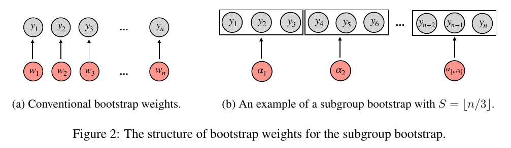
Subgroup Bootstrap

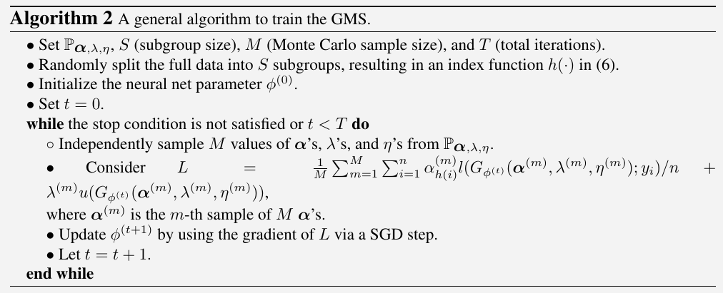
The above algorithm is analogous to the simple gradient descent method:

To solve $\hat \theta = \argmin f(\theta)$:

• Set $t = 0$ and initialize $\theta^{(0)}$
• while $t < T$
  • $\theta^{(t+1)} = \theta^{(t)} - \gamma \frac{\partial f}{\partial \theta}\mid_{\theta = \theta^{(t)}}$
  • Let $t = t + 1$
• end

So the training of MLP is just like the optimization of a function, which does not require training data ${y, \theta}$. In other words, just think it as a special function.

Structures of Generator Function

The simple MLP converges slowly for GMS and GBS applications. They modified it by a Taylor approximation of the first derivative of the weighted loss function.

Consider a weighted M-estimation loss $\sum_{i=1}^nw_i\ell(\theta; y_i)$ and its optimizer $\hat\theta_w$. Assume $\sum_{i=1}^nw_i\ell’(\hat\theta_w; y_i)=0$. With Taylor approximation,

Thus,

Propose a new NN structure called the Weight Multiplicative MLP (WM-MLP) as a sum of a simple MLP and a weight multiplicative network:

Cross-validation for LASSO

library(mvtnorm)
library(glmnet)
library(lars)
library(GMS)
set.seed(1234)
n = 500
p = 50
sigma0 = 1
beta0 = numeric(p)
beta0[1:3] = c(1, -2, 1)
Sigma = matrix(1/2, p, p) + diag(1/2, p, p)
X = rmvnorm(n, sigma = Sigma)
y = X %*% beta0 + rnorm(n) * sigma0
nfold = 10
foldid = rep(1:nfold, each=n/10)
lams = exp(seq(-9, -1, length.out = 100))
# # standardize_y
k = sqrt(var(y) * (n-1) / n)
y = y / k[1]

## #######################################
## cross-validation for lasso via glmnet
## #######################################
fit.cvlasso = cv.glmnet(X, y, alpha = 1, lambda = lams, 
                        intercept = FALSE, 
                        family = "gaussian", 
                        standardize = FALSE,
                        foldid = foldid
                        )
## ######################################
## cross-validation for lasso via lars
## ######################################
# the CV error is NOT w.r.t lambda, instead, L1 norm
# fit.cvlars = cv.lars(X, y, type = "lasso", mode = "lambda")
mycv.lasso <- function(X, y, lams) {
    nlam = length(lams)
    err = matrix(0, nfold, nlam)
    for (i in 1:nfold) {
        fit = lars(X[foldid != i, ], y[foldid != i], type = "lasso", intercept = FALSE, normalize = FALSE)
        for (j in 1:nlam) {
            yhat = predict(fit, X[foldid == i, ], lams[j] * n, mode = "lambda", type="fit")$fit
            err[i, j] = mean((yhat - y[foldid == i])^2)
        }
    }
    colMeans(err)
}
fit.cvlars = mycv.lasso(X, y, lams)

fit_GMS = GMS(X, y, model="linear", type="CV", NN_type="MLP", 
                cv_K = 10, S = n, 
                # K0 = 10, 
                K0 = n,
                num_it = 10000, lam_schd = lams * 2,
                lr0 = 0.0005, lr_power = 0.3)
samples_GMS = GMS_Sampling(fit_GMS, B1 = 1000, B10 = 1000, X = X, y = y)

plot_compare_cv = function() {
    pdf("lasso.pdf", width = 10, height=5)
    par(mfrow = c(1, 2))
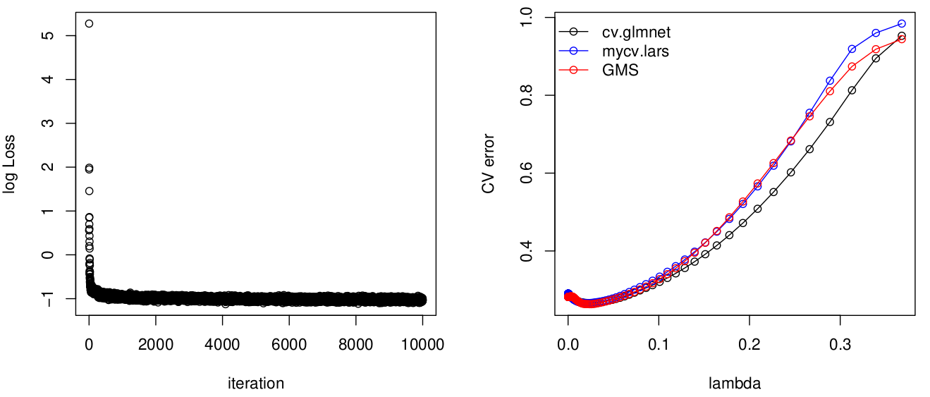
    plot(log(fit_GMS$LOSS), xlab = "iteration", ylab = "log Loss")
    ymin = min(c(min(fit.cvlasso$cvm), min(fit.cvlars), min(samples_GMS$CV_err)))
    ymax = max(c(max(fit.cvlasso$cvm), max(fit.cvlars), max(samples_GMS$CV_err)))
    plot(fit.cvlasso$lambda, fit.cvlasso$cvm, type = "o", ylim = c(ymin, ymax), xlab = "lambda", ylab = "CV error")
    points(lams, fit.cvlars, type = "o", col = "blue")
    points(samples_GMS$lam_schd / 2, samples_GMS$CV_err, col = "red", type = "o")
    legend("topleft", legend=c("cv.glmnet", "mycv.lars", "GMS"), bty="n", col = c("black", "blue", "red"), lty=1, pch=1)
    dev.off()
}

plot_compare_cv()

without standardized y, cv.glmnet does not agree with GMS and cv.lars.

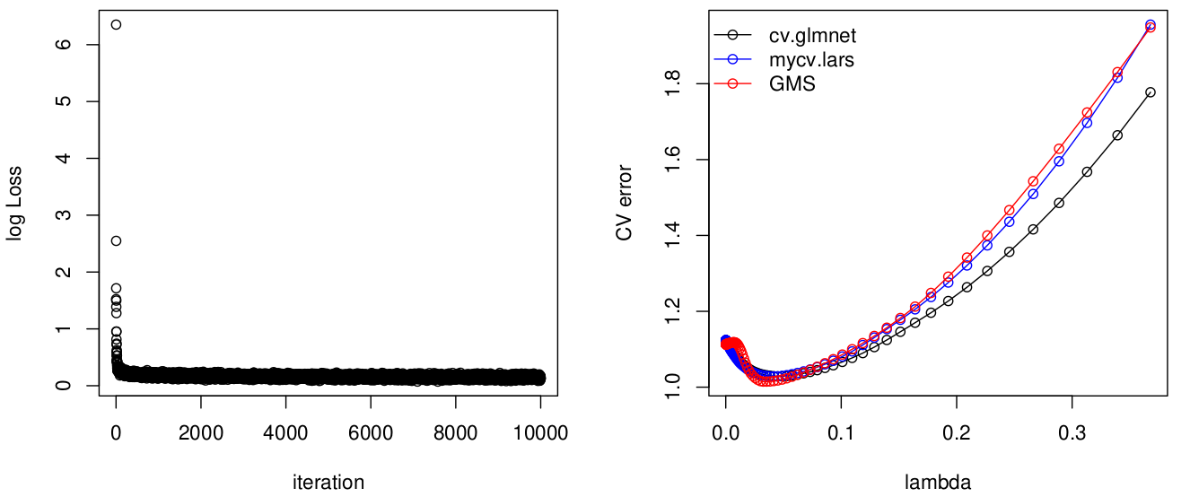
It is similar after standardizing $y$,