Monetone B-spline Smoothing

Posted on Mar 09, 2021 (Update: Mar 12, 2021) 0 Comments

Tags: B-spline, Monotone Function, Item Response Theory, Isotonic Regression, Quantile Curves, Uniform Convergence

This note is based on He, X., & Shi, P. (1998). Monotone B-Spline Smoothing. Journal of the American Statistical Association, 93(442), 643–650., and the reproduced simulations are based on the updated algorithm, Ng, P., & Maechler, M. (2007). A fast and efficient implementation of qualitatively constrained quantile smoothing splines. Statistical Modelling, 7(4), 315–328.

\[\newcommand\RMSE{\mathrm{RMSE}}\]

Introduction

There are various smoothing techniques:

• kernel smoothing
• nearest neighbors
• smoothing splines
• local polynomials
• B-spline approximation
• neural networks

Focus: estimate regression curves that are known or required to be monotone.

Examples:

• growth curves, such as weight or height of growing objects over time
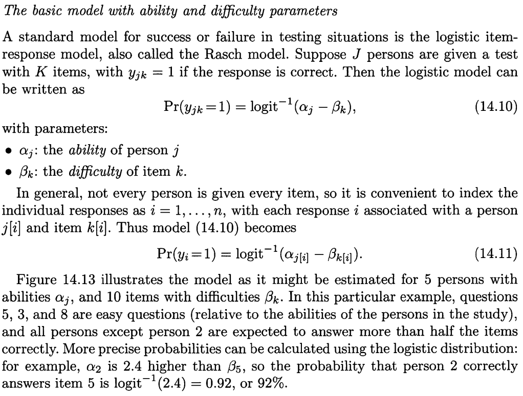
• item characteristic curve in the item response theory, which measures the probability of getting a correct answer for an examinee with given latent ability parameter.

Item-response theory (IRT) model

Isotonic regression

The paper points out that the isotonic regression undersmoothes the data and is very sensitive to outlying observations at the endpoints of the design space.

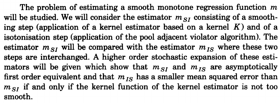
A natural idea is to combine smoothing with isotonic regression, and Mammen (1991) investigates the asymptotic performance of two different strategies,

• $m_{SI}$: first smoothing then isotonic
• $m_{IS}$: first isotonic then smoothing

$I$ splines

$I$ splines are obtained by integrating $B$ splines with positive coefficients to ensure monotonicity.

But the class of $I$ splines is relatively small compared to the class of monotone splines, and that there is always a possibilities that the fit to the data could be improved by allowing more general monotone splines.

Proposal

propose a method based on constrained least absolute deviation principle in the space of B-spline functions

• LAD: can be solved by linear programs
• $L_1$ loss function: the resulting fit approximates the conditional median function rather than the conditional mean

Method

Suppose $n$ pairs of observations ${(x_i, y_i),i=1,\ldots,n}$.

\begin{equation} y_i = g(x_i) + u_i, i=1,\ldots,n\label{eq:1} \end{equation}

w.l.o.g, restrict $x\in [0, 1]$.

Let $0 = t_0 < t_1 < \cdots < t_{k_n}=1$ be a partition of $[0, 1]$. Let $N=k_n+p=(k_n-1)+(p+1)$ and $\pi_1(x),\ldots, \pi_N(x)$. Choose quadratic splines $p=2$,

\[\pi(x) = (\pi_1(x), \pi_2(x), \ldots, \pi_N(x))\]

Estimate $g$ by $\hat g_n(x)=\pi(x)^T\hat\alpha$ by minimizing

\[\sum_{i=1}^n\vert y_i-\pi(x_i)^T\hat\alpha\vert\]

s.t. monotonicity on $\hat g_n$, or equivalently

\[\pi'(t_j)^T\alpha\ge 0, j=1,\ldots,k_n\]

Rewrite it as

\[\sum_{i=1}^n r_i^+ + r_i^-\]

subject to

\[r_i^+\ge 0, r_i^-\ge 0, r_i^+ - r_i^- = y_i-\pi(x_i)^T\alpha, i=1,\ldots,n\]

and

\[\pi'(t_j)^T\alpha\ge 0, j=0,\ldots,k_n\]

Propose a set of knots equally spaced in percentile ranks.

View the problem of choosing $k$ as model selection to minimize

\[IC(k) = \log\left(\sum_i\vert y_i-\hat g_n(x_i)\vert\right) + 2(k+2)/n\]

where the factor $2$ is selected mainly due to their experience.

a possible shortcoming is that the degree of freedom should depends on the number of ties in $\alpha$.

The monotone B-spline smoothing generalizes directly to the problem of estimating monotone quantile functions by replace $\vert \cdot \vert$ with

\[\rho_\tau(r) = r(\tau - I(r < 0))\]

some applications, satisfy certain boundary conditions, such as $0\le g(0)\le g(1)\le 1$ for a probability curve.

Asymptotic results

Assume that

• model \eqref{eq:1} holds with iid errors
• the knots $t_j$ are nonstochastic and nearly uniformly spaced

In addition, make the following assumptions

• C1: The distribution of the design points are not too far from uniform in [0, 1]. The design points $x_i\in [0, 1] (i=1,\ldots,n)$ satisfy

\[\int_0^{x_i} w(t) dt = \frac in + O\left(1/n^2\right), \; 1\le i\le n\,,\]

for some continuous function $w$ such that $\int_0^1 w(t)dt = 1$ and $0 < c_1\le w(t) \le c_2<\infty$ for some constants $c_1$ and $c_2$.

• C2: Error distribution. The distribution of $u_i$ has a uniformly bounded, continuous, and strictly positive density $f$ with a uniformly bounded derivative.
• C3: Smoothness of $g$. The regression function $g$ has a uniformly continuous $m$th ($m\ge 2$) order derivative on $[0, 1]$

Assume that conditions C1, C2, and C3 hold. If $k_n \sim (n/\log n)^{1/(2m+1)}$, then with probability one the $B$-spline estimate $\tilde g_n$ of order $m$ or $m+1$ satisfies

\[\sup_{x\in [0, 1]}\vert \tilde g_n(x) - g(x)\vert = O\left((\log n/n)^{m/(2m+1)}\right)\,,\]

and

\[\sup_{x\in [0, 1]}\vert \tilde g_n'(x) - g'(x)\vert = O\left((\log n/n)^{(m-1)/(2m+1)}\right)\,.\]

Considering the use of quadratic splines when C3 holds with $m = 2$, the rate of convergence for the constrained $B$-spline estimate $\hat g_n$ is the same as that of the unconstrained one if $g$ is strictly monotone.

Suppose that $g$ is strictly increasing. Let $\varepsilon_0 = \min{g’(x), x\in [0, 1]} > 0$. If $\tilde g_n’$ converges uniformly to $g’$, then as $n$ becomes sufficiently large, say $n > n(\varepsilon_0)$, we have

\[\vert \tilde g_n'(t_j) - g'(t_j)\vert < \varepsilon_0/2\,,\]

for all knots, then

\[\varepsilon_0/2 \le g(t_j) - \varepsilon_0/2 < \tilde g_n'(t_j) < g(t_j) + \varepsilon_0/2\]

for all knots. Because $\tilde g_n’$ is piecewise linear, this implies that $\tilde g_n$ is actually monotone (Maybe we can directly conclude by using the uniform convergence on any $x$ instead of knots). In other words, the constrained and the unconstrained $B$-spline estimates are identical when $n > n(\varepsilon_0)$. Hence, the asymptotic properties of the unconstrained $B$-spline estimate $\tilde g_n$ carry over to $\hat g_n$.

Then we directly obtain the first result in the following theorem.

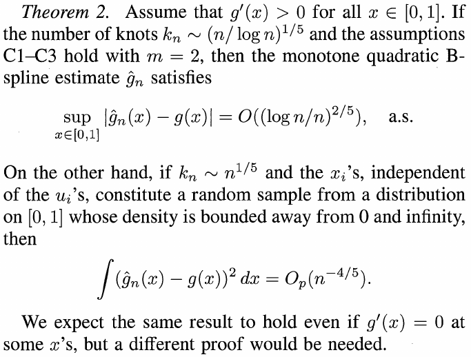
The second result comes from the He and Shi (1994),

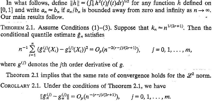
where $j = 0, r = 2$.

Simulations

Compare the root mean squared error (RMSE) with competitors

\[\RMSE(q) = \left\{(n-2q)^{-1}\sum_{i=q+1}^{n-q}(\hat g_n(x_i)-g(x_i))^2\right\}^{1/2}\]

where $q$ aims to compare the performance in the interior of the design space, and $\RMSE(0)$ is the classical $\RMSE$.

Note that the error term is calculated as $\hat g_n(x_i) - g(x_i)$ instead of $\hat g_n(x_i) - y_i$, where $y_i = g(x_i) + u_i$.

The original competitors are

• Kernel Smoothing with WARPing algorithm, which can automatically determine the bandwidth
• Monotone Kernel, which first perform isotonic regression then smoothing

I did not find available implementation for the WARPing algorithm, and then I pick the Local Polynomial Regression Fitting (loess in R), and also consider $m_{SI}$ in additional to $m_{IS}$.

The implementation of the paper’s method is calling cobs from Ng & Maechler (2007)’s COBS package.

The results are

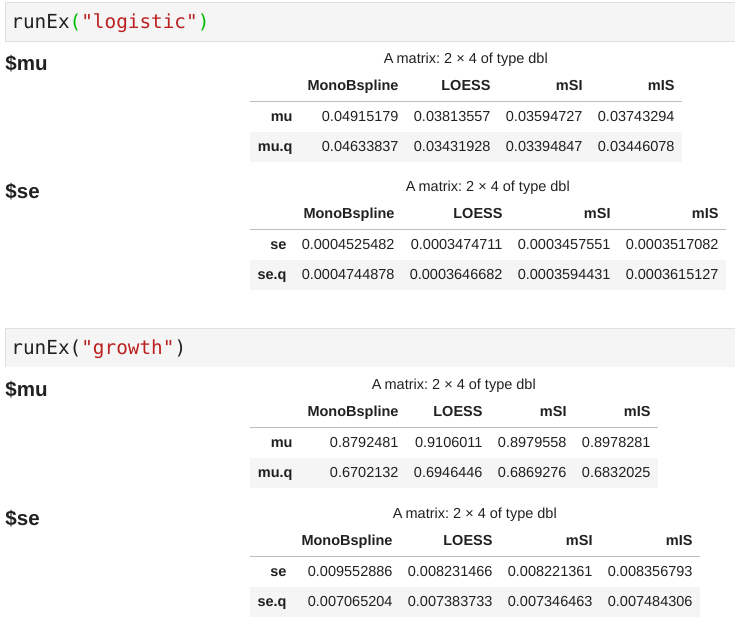
Note that the numeric results for the proposed method are quite close to the original paper.