Principal Curves
Posted on (Update: )
This post is mainly based on Hastie, T., & Stuetzle, W. (1989). Principal Curves. Journal of the American Statistical Association.
Principal curves are smooth one-dimensional curves that pass through the middle of a $p$-dimensional data set, providing a nonlinear summary of the data.
Type of summary for the pattern exhibited by the points on two variables:
- a trivial summary: the mean vector that simply locates the center of the cloud but conveys no information about the joint behavior of the two variables
- treat one of the variables as a response variable and the other as an explanatory variable.
- in many situations we do not have a preferred variable that we wish to label “response”, but would still like to summarize the joint behavior of $x$ and $y$
- an obvious alternative is to summarize the data by a straight line that treats the two variables symmetrically, and the first PC line is found by minimizing the orthogonal deviations
linear regression -> nonlinear function of $x$; similarly, a straight line -> smooth curve
Formally, define principal curves to be those smooth curves that are self-consistent for a distribution or data set. This means that if we pick any point on the curve, collect all of the data that project onto this point, and average them, then this average coincides with the point on the curve.
The largest PC line can be used in several situations
- errors-in-variables regression
- replace several highly correlated variables with a single variable
- factor analysis
and in all the previous situations the model can be written as
\[\bfx_i = \bfu_0 + \bfa\lambda_i + \bfe_i\,,\]where $\bfu_0 + \bfa\lambda_i$ is the systematic component and $\bfe_i$ is the random component.
A natural generalization is the nonlinear model,
\[\bfx_i = \bff(\lambda_i) + \bfe_i\,.\]A one-dimensional curve in $p$-dimensional space is a vector $\bff(\lambda)$ of $p$ functions of a single variable $\lambda$. These functions are called the coordinate functions, and $\lambda$ provides an ordering along the curve.
The vector $\bff’(\lambda)$ is tangent to the curve at $\lambda$ and is sometimes called the velocity vector at $\lambda$. A curve with $\Vert \bff’\Vert = 1$ is called a unit-speed parameterized curve. We can always reparameterize any smooth curve with $\Vert \bff’\Vert > 0$ to make it unit speed. Such a curve is also called parameterized by arc length since the arc length equals
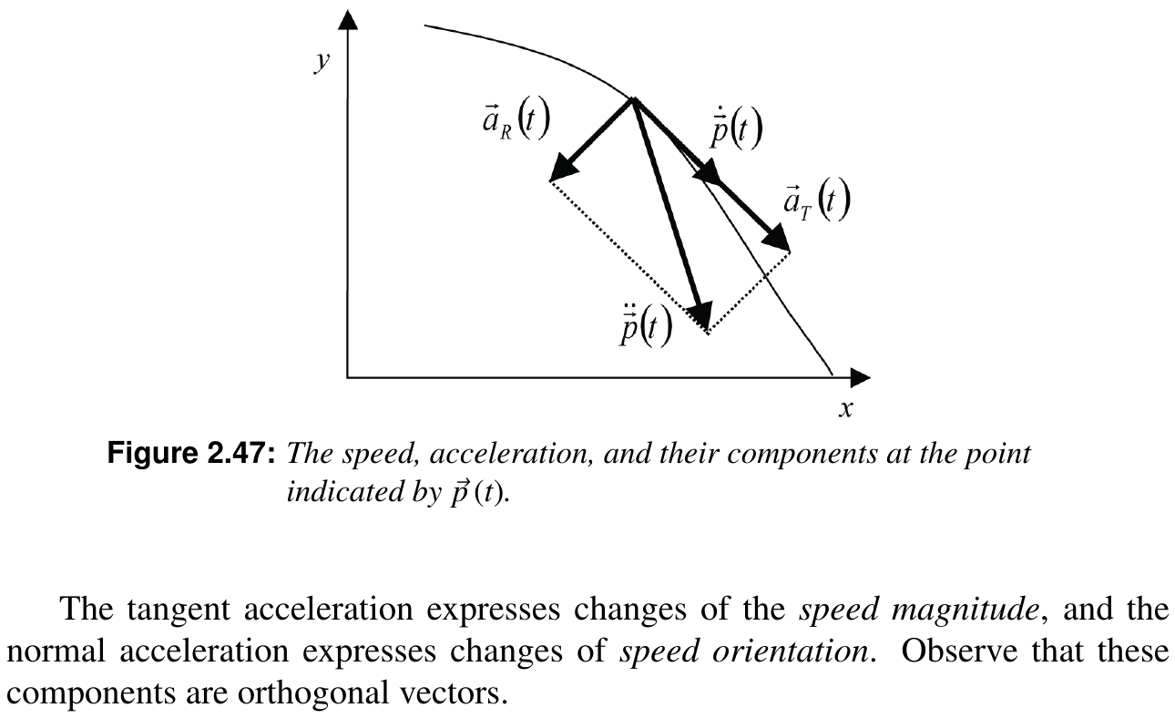
\[\int_0^\lambda\Vert \bff'(t)\Vert dt = \int_0^\lambda dt=\lambda\,.\]The vector $\bff’’(\lambda)$ is called the acceleration of the curve at $\lambda$, and for a unit-speed curve it is easy to check that it is orthogonal to the tangent vector. (TODO: to check) Here is an explanation from classical mechanics,
The acceleration is also a vector quantity typically decomposed into two components, one parallel to the speed $\bff’(\lambda)$, called the tangent acceleration, and the other a component normal to the speed, the so-called radial acceleration. Since the tangent speed is always unitary, then the tangent acceleration is zero, and hence $\bff’’(\lambda)$ is normal to the curve (i.e., normal to the tangent of the curve).
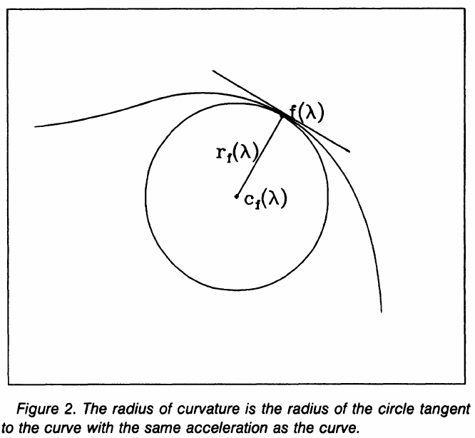
There is a unique unit-speed circle in the plane that goes through $\bff(\lambda)$ and has the same velocity and acceleration at $\bff(\lambda)$ as the curve itself. The radius $r_\bff(\lambda)$ of this circle is called the radius of curvature of the curve $f$ at $\lambda$, and $r_\bff(\lambda) = 1/\Vert \bff’’(\lambda)\Vert$.
Denote by $\bfX$ a random vector in $\IR^p$ with density $h$ and finite second moments. Without loss of generality, assume $\E(\bfX) = 0$. Let $f$ denote a smooth $C^\infty$ unit-speed curve in $\IR^p$ parameterized over $\Lambda \subset \IR^1$, a closed (possibly infinite) interval, that does not intersect itself ($\lambda_1\neq \lambda_2\Rightarrow f(\lambda_1)\neq f(\lambda_2)$) and has finite length inside any finite ball in $\IR^p$.
Define the projection index $\lambda_\bff: \IR^p\rightarrow \IR^1$ as
\[\lambda_f(x) = \sup_\lambda\{\lambda:\Vert \bfx-\bff(\lambda)\Vert = \inf_\mu \Vert \bfx-\bff(\mu)\Vert\}\]The curve $\bff$ is called self-consistent or a principal curve of $h$ if $E(\bfX\mid \lambda_\bff(X)=\lambda) = \bff(\lambda)$ for a.e. $\lambda$.
Several interesting questions:
- for what kinds of distributions do principal exist
- how many different principal curves are there for a given distribution
- and what are their properties
The principal curve is biased for the functional model $\bfX=\bff(\lambda)+\bepsilon$ with $\bff$ smooth and $E(\bepsilon) = 0$ since $\bff$ generally seems not to be a principal curve.
Connections between principal curves and principal components
- If a straight line is self-consistent, then it is a principal component
- principal components need not be self-consistent in the sense of the definition, but they are self-consistent with respect to linear regression.
A distance property of principal curves
- principal components are critical points of the distance from the observation in terms of straight line perturbations
- the principal curve is a critical point in terms of smooth curves perturbations.
Other approaches to fit nonlinear one-dimensional manifolds
- Carroll (1969): fit a model of the form $x_i = p(\lambda_i) + e_i$, where $p(\lambda)$ is a vector of polynomials functions, and the coefficients are found by linear least squares
- Etezadi-Amoli and McDonald (1983): same as Carroll’s, but use different goodness-of-fit measure
- Shepard and Carroll (1966): proceed from the assumption that the $p$-dimensional observation vectors lie exactly on a smooth one-dimensional manifold.
Bias in a simple model
Consider a unit speed curve $f(\lambda)$ with constant curvature $1/\rho$, where $\rho$ is the radius of the circle,
\[f(\lambda) = \begin{pmatrix} \rho\cos(\lambda/\rho)\\ \rho\sin(\lambda/\rho) \end{pmatrix}\]for $\lambda\in [-\lambda_f,\lambda_f]\subset [-\pi\rho,\pi\rho]$. And let $\Lambda_\theta\triangleq [-\lambda_\theta,\lambda_\theta]$.
Generate $x$ as follows:
- select $\lambda$ uniformly from $\Lambda_f$
- pick $x$ from some smooth symmetric distribution with first two moments $(f(\lambda), \sigma^2I)$.
Let $f(\lambda), \lambda\in \Lambda_f$ be the arc of a circle as described above. The parameter $\lambda$ is distributed uniformly in the arc, and given $\lambda$, $x=f(\lambda)+e$ where $e$ are iid with mean $0$ and variance $\sigma^2$. Concentrate on a small arc $\Lambda_\theta$ inside $\Lambda_f$, and assume that the ratio $\sigma/\rho$ is small enough to guarantee that all the points that project into $\Lambda_\theta$ actually originated from somewhere within $\Lambda_f$. Then
\[\E(x\mid \lambda_f(x)\in \Lambda_\theta) = \begin{pmatrix}r_\theta\\ 0\end{pmatrix}\,,\]where
\[r_\theta = r^\star \frac{\sin(\theta/2)}{\theta/2}\,,\]$\lambda_\theta/\rho = \theta/2$ and
\[r^\star = \lim_{\theta\mapsto 0}r_\theta = E\sqrt{(\rho+e_1)^2+e_2^2}\,.\]Finally $r^\star\rightarrow 0$ as $\sigma/\rho\rightarrow 0$.
Suppose $\lambda_f = \pi\rho$. (A full circle.) The radius of the circle, with the same center as $f(\lambda)$, that minimizes the expected squared distance to the points is
\[r^\star = \E\sqrt{(\rho + e_1)^2 + e_2^2} > \rho\,.\]Also $r^\star\rightarrow 0$ as $\sigma/\rho \rightarrow 0$.
For a given point $x$, the squared distance from a circle with raidus $r$ (the radial distance) is
\[d^2(x, r) = (\Vert x\Vert - r)^2\,.\]The expected drop in the squared distance using a circle with radius $r$ instead of $\rho$ is
\[\E \Delta D^2(x, r, \rho) = \E d^2(x, \rho) - \E d^2(x, r)\,.\]Condition on $\lambda = 0$, then $x=f(\lambda)+e = (\rho+e_1,e_2)$, and hence
\[\E \Delta D^2(x, r, \rho\mid \lambda = 0) = \rho^2 - r^2 + 2(r-\rho) \E\sqrt{(\rho + e_1)^2 + e_2^2}\,.\]The maximum is achieved by differentiating w.r.t. $r$,
\[\begin{align*} r^\star &= \E\sqrt{(\rho + e_1)^2 + e_2^2}\\ &=\rho\E \sqrt{(1+e_1/\rho)^2 + (e_2/\rho)^2}\\ &\ge \rho\E\vert 1+e_1/\rho\vert\\ &\ge \rho\vert \E(1+e_1/\rho)\vert\\ &=\rho\,, \end{align*}\]with strict inequality iff $\Var(e_i/\rho) = \sigma^2/\rho^2=0$.
When condition on some other $\lambda$, the system can be rotated around so that $\lambda = 0$ since the distance is invariant to such rotations, and thus for each value of $\lambda$, the same $r^\star$ maximizes $\E\Delta D^2(x,r,\rho\mid \lambda)$, and thus maximizes $\E\Delta D^2(x,r,\rho)$.
Rewrite $r^\star$ as
\[r^\star = \rho\E\sqrt{(1+\epsilon_1)^2 + \epsilon_2^2}\,,\]where $\epsilon_i = e_i/\rho, \epsilon_i\sim (0, \sigma^2/\rho^2)$. Expanding the square root expression using the Taylor’s expansion,
\[r^\star \approx \rho + \sigma^2/\rho\,,.\]Here the original paper is $\rho + \sigma^2/2\rho$, but I adopt the expansion $\sqrt{1+x} = 1+x/2+o(x)$ and note tha $\E\epsilon_1^2 =\E\epsilon_2^2 = \sigma^2/\rho^2$. Or something I missed?
To show Theorem 4.6, we first show that in a segment of size $\phi$, the expected distance from the points in the segment to their mean converges to the expected radial distance as $\phi\rightarrow 0$. Since the points are symmetrical about the radial axis, so the expectation will be of the form $(r, 0)$, so the goal is to show $r\rightarrow r^\star$ as $\phi\rightarrow 0$. The sketch of proof is
- the expected distance $\E[(x-\E(x\mid\lambda_f(x)\in \Lambda_\phi))^2\mid \lambda_f(x)\in\Lambda_\phi]$ >= the expected radial distance $\E[(x-r(x))^2\mid \lambda_f(x)\in\Lambda_\phi]$, where $r(x)$ denote the radial projection of $x$ onto the circle
- the expected distance <= the expected radial distance
Then suppose
\[\E(x\mid \lambda_f(x) = 0) = \begin{pmatrix} r^{\star\star}\\ 0 \end{pmatrix}\,.\]Since the conditional expectation minimizes the expected squared distance in the segment, it implies that a circle with radius $r^{\star\star}$ minimizes the radial distance in the segment. Since, by rotational symmetry, this is true for each such segment, then $r^{\star\star}$ minimizes
\[\E_\phi\E((\Vert x\Vert - r)^2\mid \lambda_f(x) = \phi)=\E(\Vert x\Vert - r)^2\,.\]By Lemma 4.6.1, $r^{\star\star} = r^\star$, and thus
\[\lim_{\phi\rightarrow 0} \E(x\mid \lambda_f(x) \in\Lambda_\phi) = \E(x\mid \lambda_f(x) = 0)\,.\]This is the conditional expectation of points that project to an arc of size 0 or simply a point. In order to get the conditional expectation of points that project onto an arc of size $\theta$, simply integrate over the arc:
\[\E(x\mid \lambda_f(x)\in \Lambda_\theta) = \underbrace{\int_{\lambda\in\Lambda_\theta} \E(x\mid \lambda_f(x)=\lambda) \Pr(\lambda_f(x)=\lambda\mid \lambda_f(x)\in \Lambda_\theta)d\lambda}_{\E_{\lambda_f(x)\in \Lambda_\theta}\E(x\mid \lambda_f(x) = \lambda)} =\frac{1}{\theta}\int_{\lambda\in\Lambda_\theta} \E(x\mid \lambda_f(x)=\lambda)d\lambda\,.\]Suppose $\lambda$ corresponds to an angle $z$, then
\[\E(x\mid \lambda_f(x) = \lambda ) = \begin{pmatrix} r^\star \cos(z)\\ r^\star \sin(z) \end{pmatrix}\]Thus
\[\E(x\mid \lambda_f(x)\in\Lambda_\theta) = \begin{pmatrix} \int_{-\theta/2}^{\theta/2} \frac{r^\star \cos(z)}{\theta}dz\\ \int_{-\theta/2}^{\theta/2} \frac{r^\star \sin(z)}{\theta}dz \end{pmatrix} = \begin{pmatrix} r^\star \frac{\sin(\theta/2)}{\theta/2}\\ 0 \end{pmatrix}\]Viewpoint from Mixture Model
The result of the above bias is that, suppose $\bfY$ satisfies
\[Y_j=f_j(S)+\epsilon_j;\qquad j=1,\ldots,p\,,\]where $S$ and $\epsilon_j,j=1,\ldots,p$ are independent with $E(\epsilon_j) = 0$ for all $j$.
Tibshirani, R. (1992) viewed the principal curve problem in terms of a mixture model, which avoid the above bias.
Principal curves for distributions
Let $\bfY = (Y_1,\ldots, Y_p)$ be a random vector with density $g_\bfY(y)$. Imagine that each $\bfY$ value was generated in two stages:
- generate a latent variable $S$ according to some distribution $g_S(s)$
- generate $\bfY = (Y_1,\ldots, Y_s)$ from a conditional distribution $g_{\bfY\mid s}$ having mean $\bff(S)$, with $Y_1,\ldots, Y_p$ conditionally independent given $s$
Hence, define a principal curve of $g_\bfY$ to be a triplet $\{g_S, g_{\bfY\mid S}, \bff\}$ satisfying the following conditions
- $g_S(s)$ and $g_{\bfY\mid s}(y\mid s)$ are consistent with $g_\bfY(y)$, that is, $g_\bfY(y)=\int g_{\bfY\mid s}g_S(s)ds$
- $Y_1,\ldots,Y_p$ are conditionally independent given $s$
- $\bff(s)$ is a curve in $\IR^p$ parameterized over $s\in\Gamma$, a closed interval in $\IR^1$, satisfying $\bff(s)=\E(\bfY\mid S=s)$.
Generally, HS definition and the new definition are NOT the same except in special cases. Suppose $S\sim g_s$, $\bff(s)$ is linear, and
the support of the distribution $g_{\bfY\mid s}$ is only on the projection line orthogonal to $\bff(s)$ at $s$
Then
\[E(\bfY\mid S=s) = E(\bfY\mid s_f(y) = s)\]However, the assumption is somewhat unnatural, and violates the above second condition.
Other special cases for which a curve $f(s)$ is a principal curve under both definitions:
- for a multivariate normal distribution, the principal components are principal curves under both definitions.
Principal curves for datasets
- observations: $y_i = (y_{i1},\ldots, y_{ip})$
- unobserved latent data: $s_1,\ldots, s_n$
The form of $g_S(s)$ is left completely unspecified but $g_{\bfY\mid S}$ is assumed to be some parametric family. Allow additional parameters $\Sigma(s)$ in the specification of $g_{\bfY\mid S}$ and let the complete set of unknowns be $\theta = \theta(s) = (\bff(s), \Sigma(s))$.
The log-likelihood has the form of a mixture,
\[l(\theta) = \sum_1^n\log\int g_{Y\mid S}(y_i\mid \theta)g_S(s)ds\label{eq:logll}\]A general theorem on mixtures given by Lindsay (1983) implies that for fixed $\bbf(s)$ and $\Sigma(s)$, the nonparametric maximum likelihood estimate of the mixing density $g_S$ is discrete with at most $n$ support points. Denote them by $a_1,\ldots,a_n$.
EM uses the complete data log-likelihood
\[l_0(\theta) = \sum_1^n \log g_{Y\mid S}(y_i\mid \theta(s_i))+\sum_1^n\log g_S(s_i)\]Let $w_{ik} = \Pr(s_i=a_k\mid y,\theta^0), v_k = g_S(a_k)=\Pr(s=a_k)$. Then
\[\begin{align*} Q(\theta\mid \theta^0) = \sum_{i=1}^n\sum_{k=1}^nw_{ik}\log g_{Y\mid S}(y_i\mid \theta(a_k)) + \sum_{i=1}^n\sum_{k=1}^n w_{ik}\log v_k \end{align*}\]A Gaussian form for $g_{Y\mid S}$ is most convenient and gives
\[g_{Y\mid S}(y_i\mid \theta(s)) = \prod_{j=1}^p \phi_{f_j(s),\sigma_j(s)}(y_{ij})\,.\]Maximizing $Q(\theta\mid \theta^0)$ gives
\[\begin{align*} \hat f_j(a_k) &= \frac{\sum_{i=1}^nw_{ik}y_{ij}}{\sum_{i=1}^nw_{ik}}\\ \hat\sigma_j^2(a_k) &= \frac{\sum_{i=1}^nw_{ik}(y_{ij} - \hat f_j(a_k))^2}{\sum_{i=1}^nw_{ik}}\\ \hat v_k &= \frac 1n\sum_{i=1}^n w_{ik}\,. \end{align*}\]For the log-likelihood \eqref{eq:logll},
- the log-likelihood has a global maximum of $+\infty$
- the solution is not unique
A remedy for these problem is to add a regularization component to the log-likelihood.
\[j(\theta) = l(\theta) - (c_2 - c_1) \sum_{j=1}^p\lambda_j\int_{c_1}^{c_2}[f_j(s)'']^2ds\]Comparison with Parametric spline curves
Note that the order of points are not needed, and it is determined in the fitting procedure. However, the parametric spline curves require the order of points.
A parametric spline curve in $\IR^s$ is a spline function where each $B$-spline coefficient is a point in $\IR^s$. More specifically, let $\bft = (t_i)_{i=1}^{n+d+1}$ be a knot vector for splines of degree $d$. Then a parametric spline curve of degree $d$ with knot vector $\bft$ and coefficients $\bfc=(\bfc_i)_{i=1}^n$ is given by
\[\bfg(u) = \sum_{i=1}^n\bfc_iB_{i,d,\bft}(u)\]where each $\bfc_i=(c_i^1,\ldots, c_i^s)$ is a vector in $\IR^s$.
With a Length Constraint
Kegl, B., Krzyzak, A., Linder, T., & Zeger, K. (2000) proposed a new definition.
Let the expected squared distance between $\bfX$ and $\bff$ be denoted by
\[\Delta(\bff) = E[\inf_\lambda\Vert\bfX - \bff(\lambda) \Vert] = E\Vert \bfX - \bff(t_\bff(\bfX))\Vert^2\,.\]A curve $\bff^*$ is called a principal curve of length $L$ for $\bfX$ if $\bff^*$ minimizes $\Delta(\bff)$ over all curves of length less than or equal to $L$.
Neither the HS nor this definition guarantees the uniqueness of principal curves.
Consider classes $\cS_1,\cS_2$, of curves of increasing complexity. For $k\ge 1$, let $\cS_k$ be the set of polygonal (piecewise linear) curves which have $k$ segments and whose lengths do not exceed $L$.
The empirical squared error is
\[\Delta_n(\bff) = \frac 1n\sum_{i=1}^n\Delta(\bfX_i, \bff)\]and let
\[\bff_{k, n} = \argmin_{\bff\in \cS_k} \Delta_n(\bff)\]In practice, propose a suboptimal method with reasonable complexity which also picks the length $L$ of the principal curve automatically. Also starts from the first PC, and then increase the number of segments by one by adding a new vertex to the polygonal line produced in the previous iteration.
Literature review from Ozertem & Erdogmus (2011)
- There is no proof of convergence for HS algorithm, existence of principal curves could only be proven for special cases such as elliptical distributions or distributions concentrated around a smooth curve, until Duchamp and Stuetzle (1996)
- Banfield and Raftery (1992): extend the HS principal curve algorithm to closed curves and propose an algorithm that reduces the estimation bias
- Tibshirani (1992): see above
- Delicado (1998): use another property of the principal line rather than self-consistency, which is based on the total variance and conditional means and finds the principal curve of the oriented points of the data set
- Stanford and Raftery (2000): propose anther approach that improves on the outlier robustness capacities of principal curves
- Chang and Grosh (2002): probabilistic principal curves approach uses a cubic spline over a mixture of Gaussians to estimate the principal curves/surfaces, is known to be among the most successful methods to overcome the common problem of bias introduced in the regions of high curvature
- Verbeek and coworkers (2001, 2002): used local principal lines to construct principal curves, known as K-segments and soft K-segments methods
- Vincent and Bengio (2003), Bengio et al. (2006): use a kernel density estimation based density estimate based density estimate that takes the leading eigenvectors of the local covariance matrices into account.
Many principal curve approaches in the literature, including the original HS algorithm, are based on the idea of minimizing mean square projection error. An obvious problem with such approaches is overfitting, and there are different methods in the literature to provide regularization.
- Kegl et al. (2000): provide a regularization version of Hastie’s definition by bounding the total length of the principal curve to avoid overfitting.
- Sandilya and Kulkarni (2002): define the regularization by constraining bounds on the turns of the principal curve
- principal graph algorithm (Kegl and Kryzak, 2002): can handle self-intersecting data
The paper itself defines the principal curves with no explicit smoothness constraint at all; they assume that smoothness of principal curves/surfaces is inherent in the smoothness of the underlying probability density (estimate).
Reference
- Luciano, da F. C., & Cesar Jr, Roberto Marcondes. (2009). Shape classification and analysis: Theory and practice. CRC Press, Inc.
- Kegl, B., Krzyzak, A., Linder, T., & Zeger, K. (2000). Learning and deslign of principal curves. IEEE Transactions on Pattern Analysis and Machine Intelligence, 22(3), 281–297.
- Hastie, T., & Stuetzle, W. (1989). Principal Curves. Journal of the American Statistical Association, 84, 15.
- Tibshirani, R. (1992). Principal curves revisited. Statistics and Computing, 2(4), 183–190.
- Ozertem, U., & Erdogmus, D. (2011). Locally Defined Principal Curves and Surfaces. Journal of Machine Learning Research, 12, 1249–1286.