Robust Registration of 2D and 3D Point Sets
Posted on (Update: )
This note is for Fitzgibbon, A. W. (2003). Robust registration of 2D and 3D point sets. Image and Vision Computing, 21(13), 1145–1153.
A cloud of point samples from the surface of an object is obtained from two or more points of view, in different reference frames. The task of registration is to place the data into a common reference frame by estimating the transformations between the datasets.
The error to be minimized is
\[E(a, \phi) = \sum_{i=1}^{N_d}w_i\Vert m_{\phi(i)} - T(a;d_i)\Vert^2\]In ICP-like algorithms $\phi(i)$ is chosen as the point which minimizes the distance between model and data, yielding the error function
\[E(a) = \sum_{i=1}^{N_d}w_i\min_j\Vert m_j - T(a; d_i)\Vert^2\]and finally the estimate of the optimal registration is given by minimizing over $a$
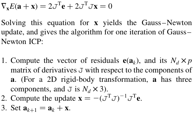
\[\hat a=\argmin_a \sum_{i=1}^{N_d}w_i\min_j\Vert m_j-T(a;d_i)\Vert^2\]The simplest ICP algorithm iterates two steps,
Beginning with an initial estimate of the registration parameters, $a_0$, the algorithm forms a sequence of estimates $a_k$, which progressively reduce the error $E(a)$. In each iteration,
- compute correspondence $\phi$: set \(\phi(i) = \argmin_{j\in\{1,\ldots,N_m\}}\Vert m_j-T(a_k;d_i)\Vert\,,\quad i=1,\ldots,N_d\)
- update transformation $a$: set \(a_{k+1} = \argmin_a\sum_{i=1}^{N_d}\Vert m_{\phi(i)} - T(a;d_i)\Vert\)
LM algorithm: rewrite
\[E(a) = \sum_{i=1}^{N_d}E_i^2(a)\]where
\[E_i(a)=\sqrt{w_i}\min_j\Vert m_j-T(a;d_i)\Vert\]and consider the vector of residuals $e(a) = \{E_i(a)\}_{i=1}^{N_d}$, then $E(a) = \Vert e(a)\Vert^2$
The LM algorithm combines the gradient descent and Gauss-Newton approaches to function minimization.
Difference between Gauss-Newton and Newton
For $f(x) = r^2(x)$, the derivatives are $f’(x)=2r(x)r’(x)$ and $f^{\prime\prime}(x)=2(r(x)r^{\prime\prime}(x)+(r’(x))^2)$. Newton’s method uses the second derivative, while Gauss-Newton uses the approximation $f^{\prime\prime}(x)\approx 2(r’(x))^2$.
It is trivial to modify the error function to include a robust kernel for LM-ICP. The kernel can be
- Lorentzian: $\epsilon(r) = \log\left(1+\frac{r^2}{\sigma}\right)$
- Huber: $\epsilon(r)=\begin{cases}r^2 & r<\sigma\\ 2\sigma\vert r\vert - \sigma^2& r\ge \sigma\end{cases}$
Fast ICP using the distance transform
The Euclidean distance transform of a set of points $\{m_j\}_{j=1}^{N_m}$,
\[D_E(x) = \min_j\Vert m_j - x\Vert\]Analogously define the $\epsilon$-distance transform $D_\epsilon$ by
\[D_\epsilon(x) = \min_j\epsilon^2(\vert m_j-x\vert)\]If the mapping $\Vert x\Vert \mapsto \epsilon^2(\vert x\vert)$ is monotonic, then $D_\epsilon(x) = \epsilon^2(\vert D_E(x)\vert)$.