Common Functional Principal Components
Posted on (Update: )
This post is based on Benko, M., Härdle, W., & Kneip, A. (2009). Common functional principal components. The Annals of Statistics, 37(1), 1–34.
One sample inference
First focus on one sample of i.i.d. smooth random functions $X_1,\ldots, X_n\in L^2[0, 1]$.
The space of $L^2[0,1]$. If $f\in L^2[0,1]$, then $f$ is Lebesgue integrable, and satisfies $\Vert f\Vert_{L^2[0,1]}^2 = \int_0^1 f^2(x)dx < \infty$. Since this norm does not distinguish between functions that differ only on a set of zero Lebesgue measure, we are implicitly identifying all such functions. The space $L^2[0, 1]$ is a Hilbert space when equipped with the inner product $\langle f,g\rangle_{L^2[0, 1]} =\int_0^2 f(x)g(x)dx$.
Assume a well-defined mean function $\mu= \E(X_i)$, and the existence of a continuous covariance function $\sigma(t, s) =\E[(X_i(t)-\mu(t))(X_i(s)-\mu(s))].$
The covariance operator $\Gamma$ of $X_i$ is given by
\[(\Gamma v)(t) = \int \sigma(t, s)v(s)ds,\quad v\in L^2[0, 1]\,.\]The Karhunen–Loève decomposition gives
\[X_i = \mu + \sum_{r=1}^\infty \beta_{ri}\gamma_r,\quad i=1,\ldots,n,\]where $\beta_{ri} = \langle X_i-\mu, \gamma_r\rangle$ are uncorrelated (scalar) factor loadings with $\E(\beta_{ri}) = 0, \E(\beta_{ri}^2)=\lambda_r$ and $\E(\beta_{ri}\beta_{ki})=0$ for $r\neq k$.

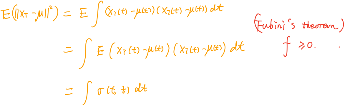
An important application is that the first $L$ principal components provide a “best basis” for approximating the sample functions in terms of the integrated square error. For any choice of $L$ orthonormal basis functions $v_1,\ldots,v_L$, the mean integrated square error
\[\rho(v_1,\ldots, v_L) = \E\left(\left\Vert X_i-\mu - \sum_{r=1}^L\langle X_i-\mu, v_r\rangle v_r\right\Vert^2\right)\]is minimized by $v_r = \lambda_r$.
The approach of estimating principal components is motivated by the well-known duality relation between row and column spaces of a data matrix.
Let $\X$ be a $n\times p$ data matrix,
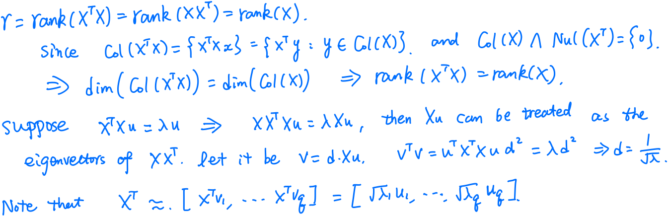
\[u_k = \frac{1}{\sqrt \lambda_k}\X^Tv_k\quad \text{and}\quad v_k = \frac{1}{\sqrt \lambda_k}\X u_k\,,\]
- The matrices $\X^T\X$ and $\X\X^T$ have the same nonzero eigenvalues $\lambda_1,\ldots,\lambda_r$, where $r = \rank(\X)$.
- The eigenvectors of $\X^T\X$ can be calculated from the eigenvectors of $\X\X^T$ and vice versa:
- The coordinates representing the variables (columns) of $\X$ in a $q$-dimensional subspace can be easily calculated by $w_k=\sqrt{\lambda_k}u_k$.
Two sample inference
For $X_1^{(1)},\ldots, X_{n_1}^{(1)}$ and $X_1^{(2)},\ldots, X_{n_2}^{(2)}$ be two independent samples of smooth functions. The problem of interest is to test in how far the distributions of these random functions coincide, which can be translated into testing equality of the different components of these decompositions
\[X_i^{(p)} = \mu^{(p)} +\sum_{r=1}^\infty \beta_{ri}^{(p)}\gamma_r^{(p)}, p=1,2\,.\]Suppose that $\lambda_{r-1}^{(p)} > \lambda_r^{(p)} > \lambda_{r+1}^{(p)}, p = 1,2$ for all $r \le r_0$ components to be considered. Without restriction, additionally assume that signs are such that $\langle \gamma_r^{(1)}, \gamma_r^{(2)}\rangle \ge 0$, as well as $\langle \hat\gamma_r^{(1)}, \hat\gamma_r^{(2)}\rangle \ge 0$.
Consider
\[H_{0_1}: \mu^{(2)} = \mu^{(2)}\quad \text{and} \quad H_{0_{2,r}}: \gamma_r^{(1)} = \gamma_r^{(2)}, r\le r_0\,.\]If $H_{0_{2,r}}$ is accepted, one may additionally want to test hypotheses about the distributions of $\beta_{ri}^{(p)},p=1,2$. If $X_i^{(p)}$ are Gaussian, then $\beta_{ri}^{(p)}\sim N(0,\lambda_r)$, then consider
\[H_{0_{3,r}}: \lambda_r^{(1)} = \lambda_r^{(2)}, \quad r=1,2,\ldots\]The corresponding test statistics are
\[\begin{align*} D_1 &\triangleq \Vert \hat\mu^{(1)} - \hat\mu^{(2)}\Vert\\ D_{2,r} &\triangleq \Vert \hat\gamma_r^{(1)} - \hat\gamma_r^{(2)}\Vert\\ D_{3,r} &\triangleq \vert \hat\gamma_r^{(1)} - \hat\gamma_r^{(2)}\vert\,. \end{align*}\,,\]and the respective null-hypothesis has to be rejected if $D_1\ge \Delta_{1;1-\alpha}, D_{2,r}\ge \Delta_{2,r;1-\alpha}$ or $D_{3,r}\ge \Delta_{3,r;1-\alpha}$, where $\Delta_{1;1-\alpha}$ denotes the critical values of the distributions of
\[\begin{align*} \Delta_1 &\triangleq \Vert \hat\mu^{(1)} - \mu^{(1)} - (\hat\mu^{(2)} - \mu^{(2)}) \Vert^2 \end{align*}\]and the critical value is approximated by the bootstrap distribution of
\[\begin{align*} \Delta_1^* &\triangleq \Vert \hat\mu^{(1)*} - \hat\mu^{(1)} - (\hat\mu^{(2)*} - \hat\mu^{(2)}) \Vert^2\,. \end{align*}\]Similarly for $\Delta_{2,r}$ and $\Delta_{3,r}$.
Even if for $r \le L$ the equality of eigenfunctions is rejected, we may be interested in the question of whether at least the $L$-dimensional eigenspaces generated by the first $L$ eigenfunctions are identical. Let $\cE_L^{(1)}$ and $\cE_{L}^{(2)}$ be the $L$-dimensional linear function spaces generated by the eigenfunctions respectively. Then test
\[H_{0_{4,L}}: \cE_L^{(1)} = \cE_L^{(2)}\,,\]which can be translated into the condition that
\[\sum_{r=1}^L \gamma_r^{(1)}(t)\gamma_r^{(1)}(t) = \sum_{r=1}^L\gamma_r^{(2)}(t)\gamma_r^{(2)}(s)\quad \text{for all }t,s\in [0, 1]\,,\]and a test statistic is
\[D_{4,L}\triangleq \int\int \left\{ \sum_{r=1}^L \hat\gamma_r^{(1)}(t)\hat\gamma_r^{(1)}(s) - \hat\gamma_r^{(2)}(t)\hat\gamma_r^{(2)}(s) \right\}^2dtds\,,\]whose critical value is also determined by the bootstrap samples.
Implied volatility analysis
European call and put options are derivatives written on an underlying asset with price process $S_i$, which yield the pay-off $\max(S_I-K, 0)$ and $\max(K-S_I, 0)$, respectively. Here
- $i$: the current day
- $I$: the expiration day
- $K$: the strike price
- $\tau = I-i$: time to maturity
The BS pricing formula for a Call option is
\[C_i(S_i, K, \tau, r, σ) = S_i\Phi(d_1) - Ke^{-r\tau}\Phi(d_2)\,,\]where $d_1 = \frac{\log(S_i/K) + (r+\sigma^2/2)\tau}{σ\sqrt{\tau}}$, and $d_2 = d_1 - σ\sqrt\tau$, $r$ is the risk-free interest rate, $\sigma$ is the (unknown and constant) volatility parameter. The Put option price $P_i$ can be obtained from the put-call parity $P_i=C_i-S_i+e^{-\tau r}K$.
The implied volatility (IV) $\tilde \sigma$ is defined as the volatility $σ$, for which the BS price $C_i$ equals the price $\tilde C_i$ observed on the market.
For a single asset, obtain at each time point $i$ and for each maturity $\tau$ a IV function $\tilde \sigma_i^\tau(K)$. For given parameters $S_i, r, K, \tau$ the mapping from prices to IVs is a one-to-one mapping.
Goal: study the dynamics of the IV functions for different maturities. More specifically, the aim is to construct low dimensional factor models based on the truncated Karhunen–Loève expansions for the log-returns of the IV functions with different maturities and compare these factor models using the above methodology.
Data: log-IV-returns for two maturity groups
- 1M group with maturity $\tau = 0.12$
- 3M group with maturity $\tau = 0.36$
Conclusion:
- the first factor functions are not identical in the factor model for both maturity groups
- none of the hypotheses for $L=2$ and $L=3$ is rejected at significance level $\alpha = 0.05$.
- in the functional sense, no significant reason to reject the hypothesis of common eigenspaces for these two maturity groups.