Soft Imputation in Matrix Completion

Posted on Apr 01, 2019

This post is based on Chapter 7 of Statistical Learning with Sparsity: The Lasso and Generalizations, and I wrote R program to reproduce the simulations to get a better understanding.

Given data in the form of an $m\times n$ matrix $\Z=\{z_{ij}\}$, find a matrix $\hat\Z$ that approximates $\Z$ in a suitable sense.

Two goals:

• gain an understanding of the matrix through an approximation $\hat\Z$ that has simple structure
• impute or fill in any missing entries in $\Z$, a problem known as matrix completion

Consider estimators based on optimization problems of the form

the constraints can be

• Sparse matrix approximation: $\Vert\hat\Z\Vert_{\ell_1}\le c$
• Singular value decomposition: $\rank(\hat\Z)\le k$
• Convex matrix approximation: $\Vert \hat\Z\Vert_*\le c$
• Penalized SVD: $\hat \Z=\U\D\V^T,\Phi_1(\u_j)\le c_1,\Phi_2(\v_k)\le c_2$
• Max-margin matrix factorization: $\hat\Z=\L\R^T,\Phi_1(\L)\le c_1,\Phi_2(\R)\le c_2$
• Additive matrix decomposition: $\hat\Z=\L+\S,\Phi_1(\L)\le c_1,\Phi_2(\S)\le c_2$

The Singular Value Decomposition

The SVD provides a solution to the rank-$q$ matrix approximation problem. Suppose $r\le \rank(\Z)$, and let $\D_r$ be a diagonal matrix with all but the first $r$ diagonal entries of the diagonal matrix $\D$ set to zero. Then the optimization problem

actually has a closed form solution $\hat \Z_r=\U\D_r\V^T$, a decomposition known as the rank-$r$ SVD.

Matrix Completion

Suppose that we observe all entries of the matrix $\Z$ indexed by the subset $\Omega \subset \{1,\ldots,m\}\times \{1,\ldots,n\}$. Given such observations, a natural approach is to seek the lowest rank approximating matrix $\hat\Z$ that interpolates the observed entries of $\Z$, namely

Generally, it is better to allow $\M$ to make some errors on the observed data as well. Consider the optimization problem,

or its equivalent form

A convenient convex relaxation of the nonconvex objective function is given by

where $\Vert \M\Vert_*$ is the nuclear norm, or the sum of the singular values of $\M$, which is also called the trace norm. The nuclear norm is a convex relaxation of the rank of a matrix.

In practice, it is unrealistic to model the observed entries as being noiseless. A more practical method is based on the following relaxed version of the program

called spectral regularization.

Soft Impute

Given an observed subset $\Omega$ of matrix entries, define the projection operator $\cP_\Omega:\bbR^{m\times n}\mapsto \bbR^{m\times n}$ as follows:

With this definition, we have the equivalence,

Given the singular value decomposition $\W=\U\D\V^T$ of a rank-$r$ matrix $\W$, define its soft-thresholded version as

Theoretical Results for Matrix Completion

• coherence constraints:
  • maximal coherence: some subset of their left and/or right singular vectors are perfectly aligned with some standard basis vector $\e_j$.
  • maximally incoherent: its singular vectors are orthogonal to the standard basis vectors

Exact Setting

Gross (2011) shows that with high probability over the randomness in the ensemble and sampling, the nuclear norm relaxation succeeds in exact recovery if the number of samples satisfies

\begin{equation}\label{eq:gross2011} N \ge Crp\log p\,, \end{equation}

where $C > 0$ is a fixed universal constant.

There is a small simulation study to better understand what the result of \eqref{eq:gross2011} saying.

1. Generate $\U,\V$ each of size $p\times r$ and with i.i.d. standard normal entries and defined $\Z=\U\V^T$.
2. Set to missing a fixed proportion of entries, and applied Soft-Impute with $\lambda$ chosen small enough so that $\Vert \cP_\Omega(\Z-\hat\Z)\Vert_F^2/\Vert \cP_\Omega(\Z)\Vert^2_F < 10^{-5}$.
3. Check to see if $\Vert \cP_\Omega^\perp(\Z-\hat\Z)\Vert_2^2/\Vert \cP_\Omega^\perp(\Z)\Vert_2^2<10^{-5}$, that is, the missing data was interpolated.

I wrote the following code to simulate with the help of softImpute package,

pr.exact.comp <- function(p = 20, r = 1, missfrac = 0.1, lam = 0.001, maxrank = r, tol = 1e-5)
{
  u = matrix(rnorm(p*r), nrow=p)
  v = matrix(rnorm(p*r), nrow=p)
  z = u %*% t(v)
  pr = p * r
  iz = seq(pr)
  imiss = sample(iz, pr*missfrac, replace = FALSE)
  zna = z
  zna[imiss] = NA
  fit = softImpute(zna, rank = maxrank, lambda = lam, type = "svd")
  #zhat = fit$u %*% diag(fit$d) %*% t(fit$v)
  zhat = complete(zna, fit)
  # check if lambda is small enough
  r1 = sum((z - zhat)[-imiss]^2) / sum(z[-imiss]^2)
  #r2 = sum((z - zhat)[imiss]^2) / sum(z[imiss]^2)
  r2 = svd((z-zhat)[imiss])$d[1]^2 / svd(z[imiss])$d[1]^2
  return((r1 < tol) & (r2 < tol))
}
sim <- function(tol = 1e-5, lam = 0)
{
  res = matrix(nrow = 10, ncol = 4)
  mf = c(0.05, 0.1, 0.15, 0.2, 0.3, 0.4, 0.5, 0.6, 0.8, 1.0)
  for (i in 1:10){
    res[i, 1] = sum(replicate(100, pr.exact.comp(p = 20, r = 1, lam = lam, missfrac = mf[i], tol = tol)))
    res[i, 2] = sum(replicate(100, pr.exact.comp(p = 20, r = 5, lam = lam, missfrac = mf[i], tol = tol)))
    res[i, 3] = sum(replicate(100, pr.exact.comp(p = 40, r = 1, lam = lam, missfrac = mf[i], tol = tol)))
    res[i, 4] = sum(replicate(100, pr.exact.comp(p = 40, r = 5, lam = lam, missfrac = mf[i], tol = tol)))
  }
  return(res)
}

res = sim(tol = 1e-4)
png("res-tol-4.png", width = 1080, height = 720, pointsize = 20)
par(mfrow = c(1, 2))
plot(mf, res[,1], type = "o", col = "orange", main = "Rank 1", 
    xlab = "Proportion Missing", ylab = "Probability of Exact Completion", ylim = c(0, 100))
lines(mf, res[,3], type = "o", col = "lightblue")
legend("topright", c("p=20", "p=40"), col = c("orange", "lightblue"), lwd = c(1,1))

plot(mf, res[,2], type = "o", col = "orange", main = "Rank 5", 
    xlab = "Proportion Missing", ylab = "Probability of Exact Completion", ylim = c(0, 100))
lines(mf, res[,4], type = "o", col = "lightblue")
legend("topright", c("p=20", "p=40"), col = c("orange", "lightblue"), lwd = c(1,1))
dev.off()

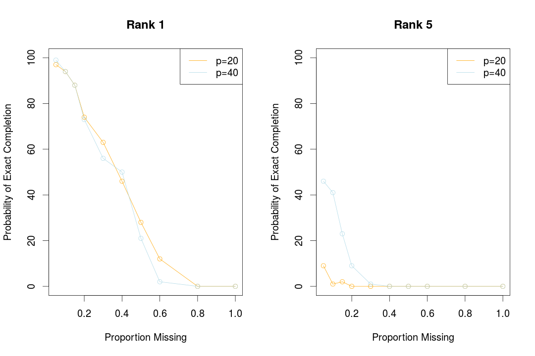
but it seems that the ratio cannot reach too much low when checking the ratio for missing part, so I adopt tol=1e-4 to get the following figure. It is important to note that, I mistook the goal of the R function softImpute, which actually cannot run for a path solution, which we need to specify by ourselves, and it indeed make some difference, but here I also try the path solution for this simulation, it still cannot work well for rank 5, which still implies that the tolerance should be larger.

Additional Noise

For the model with some additional noise,

where $\L^*$ has rank $r$. In this setting, exact matrix completion is not generally possible, and we would be interested in how well we can approximate the low-rank matrix $\L^*$ using the estimator.

Singular vector incoherence conditions are less approximate for noisy observations, because they are not robust to small perturbations.

An alternative criterion that is not sensitive to such small perturbations is based on the “spikiness” ratio of a matrix. In particular, for any nonzero matrix $\L\in \bbR^{p\times p}$, define

The ratio is a measure of the uniformity in the spread of the matrix entries.

For the nuclear-norm regularized estimator with a bound on the spikiness ratio, it can be showed that the estimate $\hat \L$ satisfies a bound of the form

with high probability over the sampling pattern, and random noise.

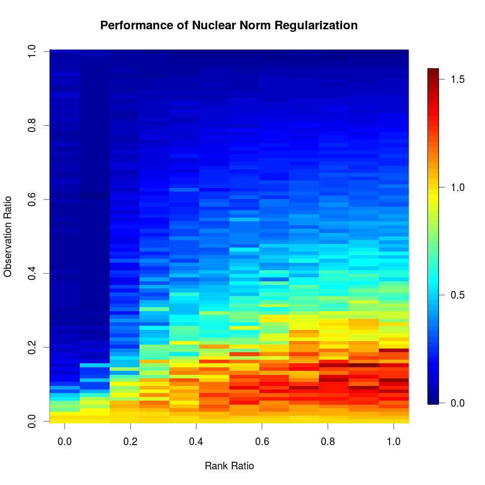
Another simulation can help us better understand the above guarantee.

• $\nu=N/p^2\in (0,1)$: the fraction of observed entries in a $p\times p$ matrix
• $\delta = r\log p/p$: the relative rank of the matrix
• $\L^*=\C\G^T$, and its noisy version $\L=\L^*+\W$

Write the following R code to do simulation,

p = 50
sigma = 1/4
sim <- function(r = 1, nu = 0.5)
{
  # generate data
  C = matrix(rnorm(p*r), nrow = p)
  G = matrix(rnorm(p*r), nrow = p)
  W = matrix(rnorm(p*p, sd = sigma), nrow = p)
  L.star = C %*% t(G)
  L = L.star + W
  # create missing
  pp = p*p
  N = pp*nu
  imiss = sample(seq(pp), pp - N, replace = FALSE)
  L.na = L
  L.na[imiss] = NA
  # perform soft-impute
  lamseq = exp(seq(from = log(2*sigma*sqrt(p*N)), to = log(1), length = 10))
  warm = NULL
  rank.max = 2
  for (i in 1:10)
  {
    fit = softImpute(L.na, lam = lamseq[i], rank = rank.max, warm = warm)
    warm = fit
    rank.max = min(sum(round(fit$d, 4) > 0)+1, 2)
  }
  L.hat = complete(L.na, fit)
  # calculate relative error
  rerr = sum((L.hat - L.star)^2) / sum(L.star^2)
  return(rerr)
}

delta = seq(from = 0, to = 1, by = log(p)/p)[-1]
nu = seq(0, 1, length.out = 101)[-1]
ndelta = length(delta)
nnu = length(nu)
res = matrix(nrow = ndelta, ncol = nnu)
for (i in 1:ndelta)
{
  for (j in 1:nnu)
  {
    res[i, j] = sim(nu = nu[j], r = i)
  }
}
png("performance-fig-7.5.png", width = 960, height = 960, pointsize = 20)
image.plot(res, xlab = "Rank Ratio", ylab = "Observation Ratio", main = "Performance of Nuclear Norm Regularization")
dev.off()

and reproduce Figure 7.5 properly,

Vignette of softImpute

Note that the mathjax cdn is invalid for the vignette of softImpute, so I quote the main description here.

Here we briefly describe the problem solved. Suppose $X$ is a large $m\times n$ matrix, with many missing entries. Let $\Omega$ contain the pairs of indices $(i,j)$ where $X$ is observed, and let $P_\Omega(X)$ denote a matrix with the entries in $\Omega$ left alone, and all other entries set to zero. So when $X$ has missing entries in $\Omega^\perp$, $P_\Omega(X)$ would set the missing values to zero.

Consider the criterion \(\min_M\frac12\|P_\Omega(X)-P_\Omega(M)\|^2_F+\lambda\|M\|_*,\) where $|M|_*$ is the nuclear norm of $M$ (sum of singular values).

If $\widehat M$ solves this convex-cone problem, then it satisfies the following stationarity condition: \({\widehat M}=S_\lambda(Z)\) where \(Z=P_\Omega(X)+P_{\Omega^\perp}(\widehat M).\) Hence $Z$ is the “filled in”” version of $X$. The operator $S_\lambda(Z)$ applied to matrix $Z$ does the following:

Compute the SVD of $Z=UDV^T$, and let $d_i$ be the singular values in $D$. Soft-threshold the singular values: $d_i^*= (d_i-\lambda)_+$. Reconstruct: $S_\lambda(Z)=UD^*V^T$. We call this operation the “soft-thresholded SVD”. Notice that for sufficiently large $\lambda$, $D^*$ will be rank-reduced, and hence so will be $UD^*V^T$. This suggests the obvious iterative algorithm: using the current estimate for $M$, create $Z$, and update $M$ by the soft-thresholded SVD of $Z$.

This is exactly what softImpute does on (small) matrices with missing values stored as NAs. By small we mean small enough that the SVD can be computed by R in a small amount of time.

This is not tenable for very large matrices, like those stored as class “Incomplete”. Here we make two very important changes to the recipe:

Re-express $Z$ at each iteration as as \(Z=P_\Omega(X)-P_\Omega(\widehat M) + \widehat M.\) This is of the form “SparseplusLowRank” (assuming $\widehat M$ is low rank), and hence can be stored. Left and right matrix multiplies by skinny matrices can also be efficiently performed. Anticipating that the solution $\widehat M$ will have low rank, compute only a low-rank SVD of $Z$, using alternating subspace methods. Indeed, softImpute has a rank argument that allows one to limit the rank of the solution; if the algorithm returns a solution with rank lower than the specified rank $r$, you know it has solved the unrestricted problem.

Consider the alternative criterion \(\min_{A,B}\frac12\|P_\Omega(X)-P_\Omega(AB^T)\|^2_F+\frac{\lambda}2(\|A\|_F^2 +\|B\|_F^2),\) where $A$ and $B$ have each $r$ columns, and let us suppose that $r$ is bigger than or equal to the solution rank of the earlier criterion. This problem is not convex, but remarkably, it has a solution that satisfies ${\widehat A}{\widehat B}^T=\widehat M$!

We can once again characterize the stationarity conditions, now in terms of $\widehat A$ and $\widehat B$. Let \(Z=P_\Omega(X)+P_{\Omega^\perp}({\widehat A}{\widehat B}^T),\) the filled in version of $X$. Then \(\widehat B= ({\widehat A}^T{\widehat A}+\lambda I)^{-1}{\widehat A}^T Z.\) We get $\widehat B$ by ridge regressions of the columns of $Z$ on $\widehat A$. For $\widehat A$ its the same, with the roles of $A$ and $B$ reversed. This again suggests an obvious alternation, now by ridged regressions. After each regression, we update the component $A$ or $B$, and the filled in $Z$. If $r$ is sufficiently large, this again solves the same problem as before.

This last algorithm (softImpute ALS) can be seen as combining the alternating subspace SVD algorithm for computing the SVD with the iterative filling in and SVD calculation. It turns out that this interweaving leads to computational savings, and allows for a very efficient distributed implementation (not covered here).