Bio-chemical Reaction Networks

Posted on Feb 25, 2019 (Update: Feb 27, 2019)

Tags: Reaction Network, Text Mining, Survey

This note is based on Loskot, P., Atitey, K., & Mihaylova, L. (2019). Comprehensive review of models and methods for inferences in bio-chemical reaction networks.

Abstract

1. key processes in biological and chemical systems are described by networks of chemical reactions.
2. parameter and state estimation in models of (bio-) chemical reaction networks (BRN)

statistical inference:

• model calibration
• discrimination
• identifiability
• checking
• optimum experiment design
• sensitivity analysis
• bifurcation (分叉点) analysis

Aim of this review:

• what BRN models are commonly used in literature
• for what inference tasks and inference methods

Method

• 700 publications in computational biology and chemistry
• 260 research paper and 20 graduate theses
• paper selection as text mining using scripts to automate search for relevant keywords and terms
• outcome tables revealing the level of interest in different inference tasks and methods for given models in literature as well as recent trends
• a brief survey of general estimation strategies to facilitate understanding of estimation methods for BRNs

findings

• many combinations of models, tasks and methods are still relatively sparse, representing new research opportunities to explore those that have not been considered
• most common models of BRNs in literature
  • differential equations
  • Markov processes
  • mass action kinetics
  • state space representations
• most common tasks in cited paper
  • parameter inference
  • model identification
• most common methods
  • Bayesian analysis
  • Monte Carlo sampling strategies
  • model fitting to data using algorithms
• future research directions

Introduction

Biological systems are presently subject to extensive research efforts to ultimately control underlying biological processes.

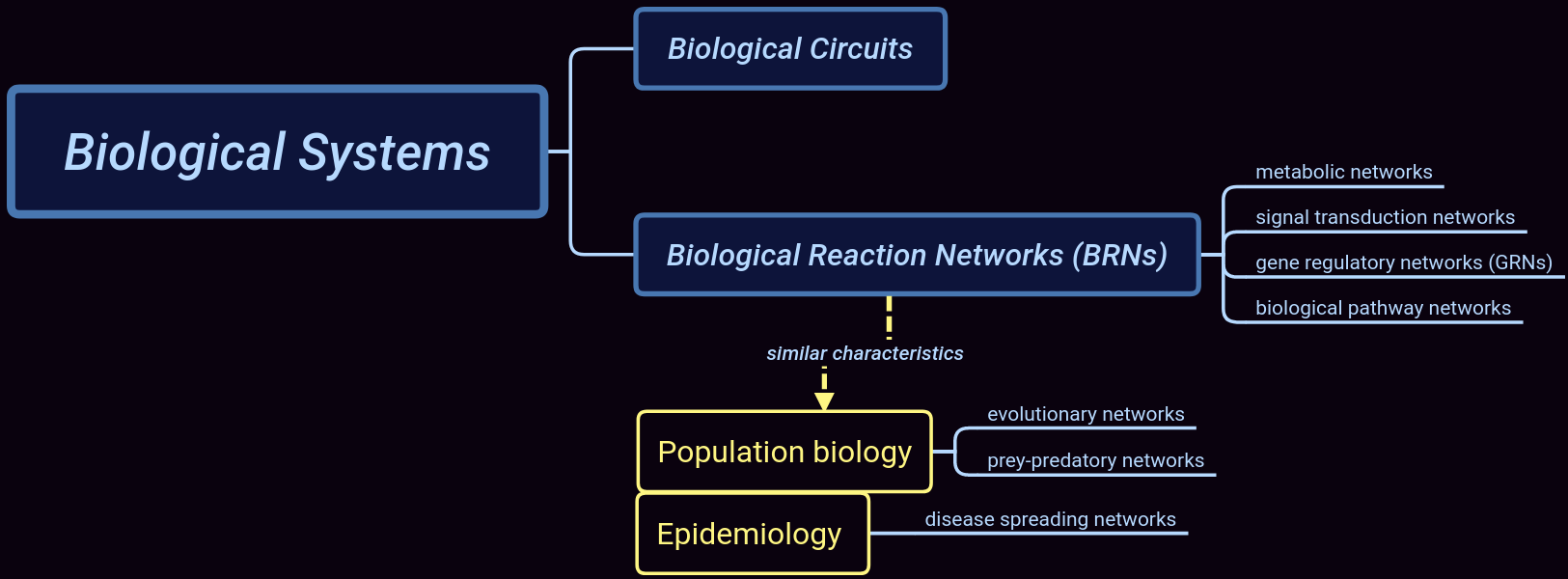
Biological systems are

• non-linear
• dynamic
• stochastic

Their responses to input perturbations is often difficult to predict as they may respond differently to the same inputs.

Biological phenomena must be considered at different spatio-temporal scales from single molecules to gene-scale reaction networks.

Biological phenomena cna be studied by elucidating properties of their mathematical models.

• Forward modeling: only collect observations which are necessary to formulate and test some biological hypothesis than to perform extensive time consuming and expensive laboratory experiments
• Reverse modeling: finding parameter values to reproduce observations, and can be enhanced by experiment design.

Models should at the right level of coarse grain description:

• microscopic stochastic models may be computational expensive
• deterministic macroscopic description such as population-average modeling may not be sufficiently accurate or have low resolution.

Model analysis is performed to find transient responses of dynamic systems, to obtain their behavior at steady-state or in equilibrium, and to explore complex multi-dimensional parameter spaces.

For many biological models, viable parameter values form only a small fraction of overall parameter space, so identifying this sub-volume by ordinary sampling would be inefficient. Other challenges include size of state space, unknown parameters, analytical intractability and numerical problems. Evaluation of observation errors can both facilitate as well as validate the analysis.

Most analytical and numerical methods can be used universally for different model structures. Efficiency of analysis:

• in statistical sense, robust against uncertainty in model structure and parameter values under noisy and limited observations.
• in computational sense, efficiency can be achieved by developing algorithms which are prone to massively parallel implementation

Concern: parameter inference in biological and chemical systems described by various BRN models

1. parameter inference is also referred to as inverse problem, point estimation, model calibration and model identification.
2. machine learning methods became popular as an alternative strategy to learn not only model parameters, but also features from labeled or unlabeled observations.
3. the key objective of parameter inference is to define, and then minimize the estimation error while suppressing the effect of measurement errors.

Parameter inference is affected by many factors:

• different models have different degree of structural identifiability.
• parameters cannot be identified or only partially identified, provided that different parameter values or different inputs generate the same dynamic response such as distributions of synthesized molecules.
  • in some cases, structural identifiability can be overcome by changing modeling strategy, structural identifiability is a necessary but not sufficient condition for overall identifiability
  • practical identifiability (also known as posterior identifiability) is defined to assess whether there are enough data to overcome measurement noise
  • it may be beneficial to test identifiability of parameters which are of interest prior to their inference.

sensitivity analysis can complement as well as support parameter estimation

• parameters can be ranked in the order of their importance, from the most easy to the most difficult to estimate
• parameters can be screened using a small amount of observations to select those which are identifiable prior to their inference from a full data set.
• other tasks in sensitivity analysis include prioritizing and fixing parameters, testing their independence, and identifying important regions of their values.

main objective: survey models and methods which are used for parameter inferences in BRN

Methodology

Identifying and selecting the most relevant papers

1. Phase I: almost 700 electronic documents
2. Phase II: reduce to 300 by defining rules and using text mining

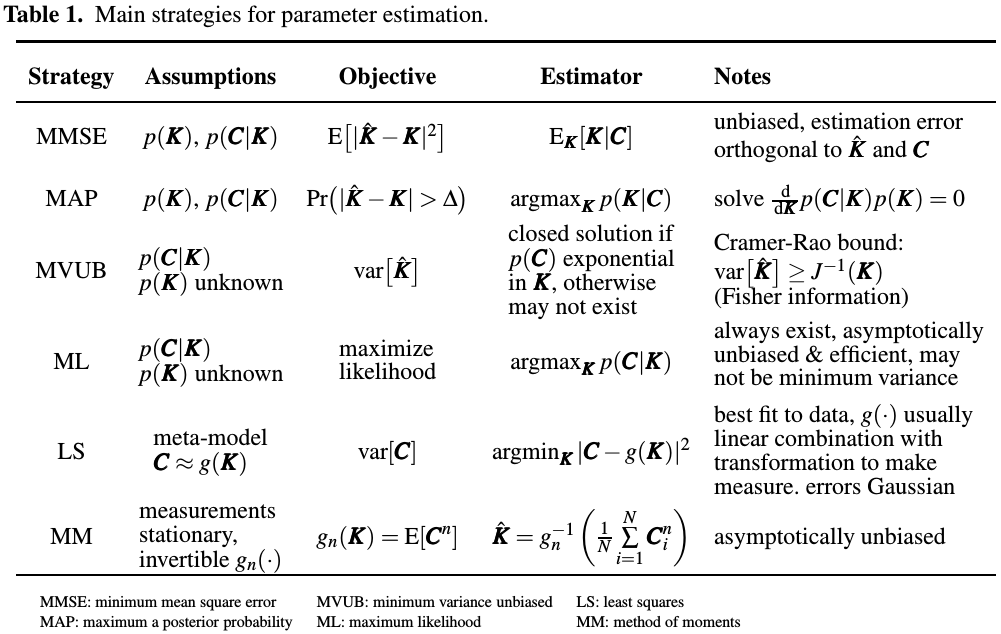
Review of General Estimation Strategies

To review general strategies of parameter estimation, and highlight assumptions limiting their use.

The measurements are noisy, and they are obtained at discrete time instances. Important assumption for choosing estimation strategy is whether the dependency of measurements on parameter values is known or only partially known.

Basic estimation problem:

• $K$: a vector of reaction rates
• $C$: kinetic parameters to be estimated from observed concentrations (or equivalently, molecule counts)

\[C_t = f(C_{t-1},\tilde C_{t-1}, K, \tilde K, w_t) = f(C_{t-1}, \tilde C_{t-1}, K, \tilde K)+w_t\,,\]

where $\tilde C$ denotes unobserved concentrations. It assumes dependency only between two successive concentration measurements. Such Markov chain assumption is normally satisfied for all BRNs. The measurement noise $w$ is additive and independent from value of concentrations and kinetic parameters, which is a somewhat strong assumption.

At time $t$, parameter values are estimated from all measurements collected so far,

\[\hat K_t = g(C_t,C_{t-1},\ldots,C_1)\,.\]

Unlike Markovian assumption, all measurements may affect estimated values.

In general, all estimators are designed to minimize some penalty function $q(\hat K, K)$. Another simplifying approximation is to assume that concentrations are continuous functions of time, even though reactions are occurring at discrete time instances.

Several criteria for selecting a suitable estimator:

1. prior pdf of $K$
2. system model may be only be partially known.
3. parameters may be time-varying.

Main strategies for parameter estimation are summarized as follows:

Various types of evolutionary algorithms such as

• genetic algorithm
• simulated annealing
• ant colony optimization
• particle swam optimization

Main issue of these numerical methods is how to determine initial estimates, the speed of convergence, how easy they can implemented, and if they are derivative free.

Other estimators:

• BLUE: require linear model of measurements,
• KF: require linear model of measurements and assumes that measurement and process noises are Gaussian
  • EKF: use first-order linearization about predicted value of parameter.
  • AKF: use second order linearization
  • UKF: represents distribution of parameter to be estimated by a group of random samples followed by unscented transformation to make them Gaussian.
• MCMC/SMC/KF: very universal and require no assumptions about system model or its parameters

In general, all sampling based estimators such as UKF, MCMC, SMC and PF are negatively affected by non-smooth non-linearities and systems involving large number of dimensions.

EM: alternative method for iteratively calculating posterior distribution (MAP) or likelihood (ML estimate)

Different implementations of EM method may involve naive Bayes strategy, and Baum-Welch or inside-outside algorithm

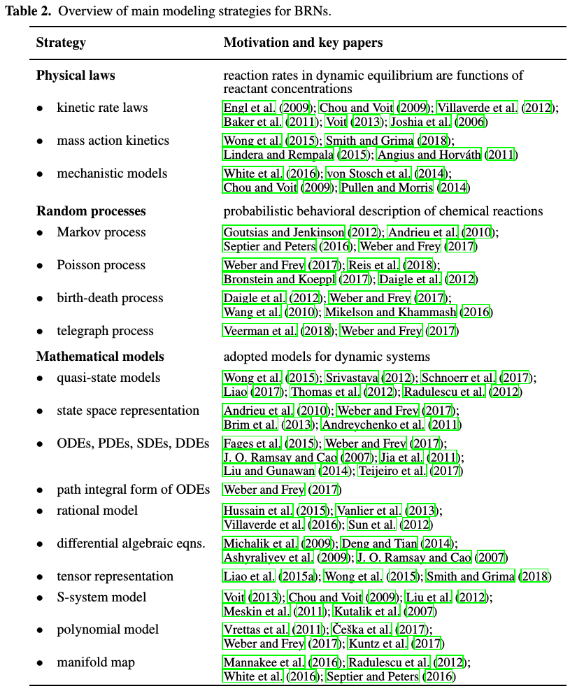
Review of Modeling Strategies for BRNs

Mathematical models describe dependencies of observations on model parameters.

Parameter estimation can be assumed together with discriminating among several competing models.

Two main physical laws considered for modeling BRNs are:

• the rate law
• the mass action law

Chemical reactants in dynamic equilibrium are governed by the law of mass action whereas kinetic properties of BRNs are described by the rate laws.

BRNs can be modeled as a sequence of reactions occurring at random time instances. Such stochastic kinetics mathematically correspond to a Markov jump process with random state transitions between the species counts. Alternatively, sequence of chemical reactions can be viewed as a hidden Markov process.

Random occurrences of reactions can be also described using a hazard function.

The number of species and their molecule counts can be large, so state space of CTMC model can be huge (Angius and Horváth, 2011). Large state space can be truncated by considering only states significantly contributing to the parameter likelihood.

(Angius and Horváth, 2011)

Consider a continuous time Markov chain describing the interaction of $M$ reagents through $R$ reactions.

Parameter likelihoods can be updated assuming increments and decrements of the species counts.

Modeling BRNs by differential equations

Time evolution of states with probabilistic transitions is described by chemical master equation (CME). It is a set of coupled first-order ODEs or partial differential equations (PDEs) representing a continuous time approximation and describing BRN quantitatively.

1. ODE model of BRN can be also derived as a low-order moment approximation of CME.
2. it is often difficult to find transition probabilities
3. the PDE approximation can be obtained assuming Taylor expansion of CME.

If deterministic ODEs cannot be solved analytically, one can use Langevin and Fokker-Planck equations as stochastic diffusion approximations of CME.

CLE is a SDE consisting of deterministic part describing slow macroscopic changes, and stochastic part representing fast microscopic changes which are dependent on the size of deterministic part.

Modeling BRNs by approximations

A popular strategy to obtain computationally efficient models is to assume approximations, for example, using meta-heuristics and meta-modeling.

• QSS
• QE

moment closure methods leading to coupled ODEs can approach CME solution with a low computational complexity. Specifically, the $n$-th moment of population size depends on its $(n+1)$ moment. In order to close the model, the $(n+1)$-th moment is approximated by a function of lower moments.

the leading term of CME approximation in system size expansion (SSE) method corresponds to linear noise approximation (LNA). It is the first order Taylor expansion of deterministic CME with a stochastic component where transition probabilities are additive Gaussian noises.

LNA is used to approximate fast reactions as continuos time Markov process whereas slow reactions are represented as Markov jump process with time-varying hazards.

Other variants of LNA:

• restarting LNA model
• LNA with time integrated observations
• LNA with time scale separation
• LNA for reaction-diffusion master equation

Other model:

• S-system model
• Polynomial models of biological systems

Other models of BRNs

• Birth-death process: a special case of CTMP having only two states
• Sloppy models

Review of Parameter Estimation Strategies for BRNs

• structural identifiability (or model identifiability): determine which parameter values can be estimated from observations.
• practical identifiability: accounts for quality and quantity of observations, whether it is possible to obtain good parameter estimates from noisy and observations.

All parameter estimation problems lead to minimization or maximization of some fitness function. Deriving optimum value analytically is rarely possible whereas numerical search for the optimum in high-dimensional parameter spaces can be ill-conditioned when objective or fitness function is multi-modal.

Parameter estimation can be facilitated by grouping parameters and identifying which are uncorrelated. Parameter estimation in groups can provide robustness against noisy and incomplete data. Only parameters which are consistent with measured data can be selected and jointly estimated.

• Akaike information
• Fisher Information
• Mutual information
• Cross-entropy methods
• Sum of squared errors

Bayesian methods

• MAP estimate
• Approximate Bayesian Computation (ABC): the basic idea is to find parameter values which generate the same statistics as the observed data.
• ABC method can be performed sequentially, and it can be coupled with sensitivity analysis.
• EM, MCEM, variational Bayesian inference
• ML estimation, likelihood function can be approximated analytically using Laplace and B-spline approximations.

Monte Carlo methods

• MCMC
• SMCMC
• CDIS
• Bayesian inference via MC sampling with stochastic gradient descent
• MCMC sampling for mixed-effects SDE
• bootstrapped MC
• SMC
• pMCMC

Other statistical methods

• standard Kalman filter
• EKF

Model fitting methods

sensitivity to initial values can be reduced by methods tracking multiple points

Evolutionary algorithms are the most frequently used methods for solving high-dimensional constrained optimization problems. EAs adopt heuristic strategies to find the optimum assuming a population of candidate solutions which are iteratively improved by reproduction, mutation, crossover or recombination, selection and other operations until fitness or loss function reaches the desired value.

• cuckoo search
• non-linear simplex method
• semi-definite programming
• Nelder-Mead method
• Machine Learning
• Deep Learning

Choices of Models and Methods for Parameter Estimation in BRNs

the most popular models for parameter inference and other related tasks are generally models involving differential equations, Markov processes, and state space representations.

the second most popular group of models for parameter estimation include S-system and polynomial models, and moment closure and linear noise approximations.

Variational Bayesian and ABC methods are mostly used with Markov processes, since this is where they were originally developed whereas Markov processes are derived from differential equations.

Future research problems

a guideline to define new problems which have not been sufficiently investigated in literature.

not forget that the ultimate goal of statistical inferences in models of BRNs is to elucidate understanding of in vivo and in vitro biological systems.

Conclusion

Aim: explore how various inference tasks and methods are used with different models of BRNs. Capture dependency between tasks, methods and models.

Common models of BRNs and inference tasks and methods were identified by text mining all cited papers.

The most common inference tasks are concerned with identifiability, parameter inference and sensitivity analysis., The most common inference methods are Bayesian analysis using MAP and ML estimators, MC sampling techniques, LS, and evolutionary algorithms for data fitting.

Access the levels of interest in different inference tasks.