SMC for Protein Folding Problem

Posted on Feb 23, 2019 (Update: Mar 09, 2019)

Tags: Protein Folding, Sequential Monte Carlo

This note is based on Wong, S. W. K., Liu, J. S., & Kou, S. C. (2018). Exploring the conformational space for protein folding with sequential Monte Carlo. The Annals of Applied Statistics, 12(3), 1628–1654.

Abstract

Background

1. computation methods are vital important for protein structure prediction from amino acid sequence, such as protein design in biomedicine.
2. efficient sampling of conformations according to a given energy function remain a bottleneck, yet is a vital step for energy-based structure prediction methods.
3. although the Protein Data Bank of experimentally determined 3D protein structures has steadily increased in size, structure predictions for new proteins tend to be unreliable in the amino acid segments where there is low sequence similarity with known structures.

Proposal

1. introduce a new method for building such segments of protein structures, inspired by sequential Monte Carlo methods.
2. apply method to examples of real 3D structure predictions and demonstrate its promise for improving low confidence segments.
3. provide applications to the prediction of reconstructed segments in known structures, and to the assessment of energy function accuracy.
4. the method is able to produce conformations that both have low energies and good coverage of the conformational space and hence can be a useful tool for protein design and structure prediction

Introduction

1. Christian B. Anfinsen (1973) proposed that the stable 3D structure of a protein is essentially determined by its amino acid sequence.
2. Since then, the question of how a protein, consisting of a linear sequence of amino acids, acquires that stable 3D structure has come to be known as the protein folding problem, and has challenged scientists of many disciplines for about a half-century.
3. The traditional way to determine a protein’s 3D structure is by laboratory work, such as crystallography.
4. Computational approaches for protein structure prediction from amino acid sequence have been developed since the advent of computers, yet many unsolved challenges remain. Further advances in the efficiency and accuracy of computational structure prediction algorithms are in critical need.

The sequence-to-structure correspondence

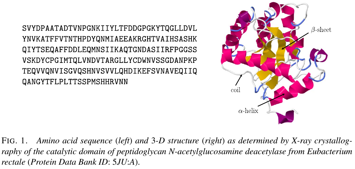
• $\alpha$-helix
• $\beta$-sheet
• coil

The energy landscape

A conformation refers to a specific arrangement of the atoms of a protein in 3D space.

A powerful approach for structure prediction is to assume that the true (or native) conformation of a protein is the one with minimum potential energy. This is based on the energy landscape theory, and accordingly, many computational methods make their predictions according to an energy function. The structure with the lowest energy value found is selected as the prediction.

Two main interconnected challenges associated with this approach:

• the energy function: physics based or fitted from data
• the search method: the focus of this paper, is to find the minimum energy conformation for a given energy function.

Many proteins of interest are composed of 100-600 amino acids, with corresponding geometric degrees of freedom numbering from several hundreds to a few thousand. Thus given the large degrees of freedom, a deterministic energy minimization approach or a direct search for the minimum is impractical.

The protein data bank for building 3D structure predictions

The homology modeling approach was developed to leverage these data and make 3D structure predictions based on sequence alignments.

Searching for minimum energy conformations

For any realistic energy function, the energy landscape of the conformational space will also be both multimodal and of high dimension. It would be very ineffective to perform energy minimization routines from arbitrary starting conformation, as such a procedure would in general yield only local minima far from the global one.

Obtaining conformations with low energies from an initial search is therefore very important and is the primary motivation for the methodology in this paper. This paper formulates the problem as the stochastic optimization of a high-dimensional distribution subject to constraints.

Since a protein is composed of a sequence of amino acids, it has been natural to consider sampling and optimization methods that exploit this sequential character. Segments of proteins can be built one amino acid at a time, and the successive steps can be designed to favor low-energy conformations.

The method

The goal is to efficiently explore the conformational space for a continuous segment of amino acids within a protein, to minimize its energy.

Propose a novel approach that combines sequential construction with inspiration from SMC.

To avoid degeneracy in the particle population, the paper makes substantive modifications to the basic sequential importance sampling scheme for this purpose.

Statistical Formulation

Protein geometry

Representation:

• a list of 3D Cartesian coordinates of the positions of each atom
• in terms of geometric degrees of freedom, which are primarily dihedral angles; bond lengths and bond angles exhibit very little variation in real structures, and fixed them at their ideal values

The backbone of a protein consists of the interconnected sequence of $\mathrm N$, $\mathrm C_\alpha$, $\mathrm C$ and $\mathrm O$ atoms for each amino acid, as follows:

free dihedral angles $(\phi,\psi,\omega)$:

• $\phi$: the distance between the C atoms of successive amino acids.
• $\psi$: N atoms
• $\omega$: $\mathrm C_\alpha$.

The side chain of an amino acid that extends from its $\mathrm C_\alpha$ atom is unique, and thus characterizes each of the 20 different amino acid types.

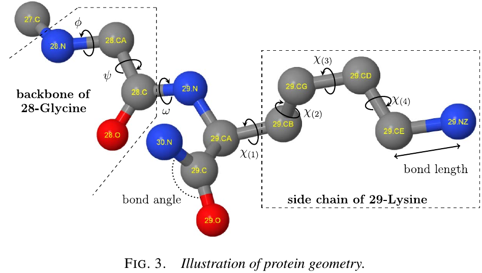
• $\chi$: position of side chain atoms for an amino acid can likewise be parameterized; there are 0 to 4 of these depends on the amino acid type.

Representation of protein segments and energy functions

a continuous segment of length $l$

$a_1,\ldots,a_l$ denote the sequence of amino acids of that segment with the rest of the structure held fixed.

two ends of the segments are anchored by fixed positions of the $\mathrm C_\alpha$ atom of $a_1$ and the $\mathrm C$ atom of $a_l$.

$(\phi_i,\psi_i,\omega_i,\chi_i)$ for $i=1,\ldots,l-1$ and $\chi_l$. for convenience, let $\chi_i$ denote the length 0-4 vector of side chain dihedral angles of amino acid $i$ (length depending on the amino acid type)

conformations for the segment must seamlessly connect to the two anchors with realistic bond lengths and angles.

the empirical distributions of the angle pairs $(\phi_i,\psi_i)$ for each amino acid type: Ramachandran plot

grouping the $(\phi_i,\psi_i)$ pairs according to secondary structure shows that the distributions for $\alpha$-helices and $\beta$-sheets are tightly constrained due to their regular angular patterns; in contrast, an amino acid located in a coil will have a much wider range of possible dihedral angles.

$\omega$ is typically close to 180 degree and hence has less effect on the backbone shape compare to $(\phi,\psi)$.

The value of $\chi$ in real structures tend to cluster around a discrete set of modes, known as $rotamers$.

• $H$: the energy function
• $x$: the vectors of all free dihedral angles of the segment

wish to find the global minimum of $H$ by stochastically searching the conformational space guided by the Boltzmann distribution

\[\pi(x)\propto \exp\{-H(x)/T\}\]

where $T$ is the effective temperature.

A generic form:

\[H(x) = H_\theta(x) + H_d(\{r_{ab};x\})\,,\]

where $H_\theta$ is the energy of the dihedral angles $x$, and $H_d$ is the energy of all pairwise distances $r_{ab}$ between atoms (i.e., atomic interactions), whose positions have been calculated based on $x$.

$H_d$ is much more costly to compute than $H_\theta$ in general.

steric clash: a pair of atoms are too close in space than can be possible in real structures (i.e., $r_{ab}$ is below a certain threshold, depending on atom types. For convenience we shall simply say $H_d=+\infty$ when there is at least one steric clash.

Since the dimension of $x$ will generally be $\ge 20$ for any realistic scenario where the method would be applied (i.e. $l\ge 8$), the sampling becomes a difficult task due to the large space and multimodality.

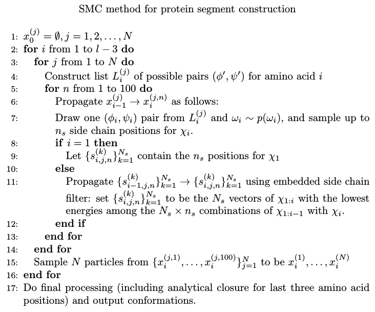
Method

A novel adaptations to the SIS scheme.

1. design a proposal $q_i$ for the propagation step that incorporates the necessary energy calculations to help ensure that the extensions of each particle $x_i^{(j)}$ conditional on $x_{i-1}^{(j)}$ do not become degenerate. This entails expending additional computational effort to evaluate $\Delta H_d$ systematically over a $(\phi_i,\psi_i)$ grid.
2. choose to propagate a much larger number of proposals from each particle, that is, $x_{i-1}^{(j)}\rightarrow (x_i^{j,1},\ldots, x_i^{(j,100)})$, thus greatly increasing the size of an intermediate particle population. Then $N$ particles can be selected as representatives from this larger intermediate population.
3. to handle the difficulty of sampling side chain angles and evaluating their energy along with $(\phi_i,\psi_i,\omega_i)$, embed a second particle filter within the main sampling steps for handling $\chi_i$.

Notation:

• $\Delta H(x\mid x’)$: the incremental energy contribution of the additional atoms corresponding to $x$ when some previous angles $x’$ have already been sampled. For protein segments, let the incremental distributions correspond to adding one amino acid at a time.
• $x_i\equiv (\phi_{1:i}, \psi_{1:i}, \omega_{1:i}, \chi_{1:i})$.
• $y_i\equiv (\phi_{1:i}, \psi_{1:i}, \omega_{1:i})$

Choice of proposal distribution $q_i$ for growth of backbone

Using 5° intervals of $\phi$ and $\psi$ angles provided sufficient resolution to reproduce protein backbones in the PDB with negligible error. This suggests that evaluating $\Delta H_d(\{r_{ab};\phi_i,\psi_i,\omega_i\}\mid y_{i-1}^{j})$ with $(\phi_i,\psi_i)$ on a 5° by 5° grid and $\omega_i=180$° would be suitable at the $i$-th propagation step, in regions where $(\phi_i,\psi_i)$ has nonnegligible probability density, that is, $\exp[-\Delta H_\theta(\phi_i,\psi_i\mid x_{i-1}^{(j)})] > \varepsilon$.

Lookahead strategy: Evaluate $\Delta H_d(\{r_{ab};\phi_{i+1},\psi_{i+1}\}\mid \phi’,\psi’, \omega_i,y_{i-1}^{(j)})$ where $(\phi_{i+1},\psi_{i+1})$ takes values on a very coarse 30 degree grid. The coarser grid is faster to evaluate and suffices to provide a rough assessment of whether backbone growth can continue successfully.

In summary, yield a list $L_i^{(j)}$ of grid points $(\phi’,\psi’)$ that are potentially good candidates for extending the particle to the $i$-th amino acid. Set $q_i(x_i\mid x_{i-1}^{(j)})\propto \1[(\phi_i,\psi_i)\in L_i^{(j)}]p(\omega_i)p(\chi_i)$.

Question: do they change their $w_i.$

Selection of $N$ particles for further backbone growth

To fully leverage the energy calculations already performed, make multiple draws from $q_i$ for each particle $j$, so that we propagate $x_{i-1}^{(j)}\rightarrow (x_i^{(j,1)},\ldots, x_i^{(j,100)})$.

To encourage diversity, making draws from $q_i$ sample grid points $(\phi_i,\psi_i)$ from the list $L_i^{(j)}$ without replacement, and we have a much larger intermediate particle population $\{x_i^{(j,1)},\ldots,x_i^{(j,100)}\}_{j=1}^N$. Then, rather than calculating weights for each particles (SIS) or resampling particles based their weights (SIR), we shall instead aim to obtain a particle population $x_i^{(1)},\ldots,x_i^{(N)}$ by suitably sampling a subset of $\{x_i^{(j,1)},\ldots,x_i^{(j,100)}\}_{j=1}^N$ that encourages low energy and high diversity.

Suppose we have evaluated the energies of all the intermediate particles, $\{H(x_i^{(j,1)}),\ldots,H(x_i^{(j,100)})\}_{j=1}^N$, where we obtain each according to

\[H(x_i^{(j,n)}) = H_\theta(y_i^{(j,n)}) + H_d(\{r_{ab};y_i^{(j,n)}\}) + H(\chi_{1:i}\mid y_i^{(j,n)})\,.\]

Within the intricate atomic environment of protein structures, growth is rather unpredictable: the eventual completed conformations with the lowest energies may not have been the lowest energy particles at the earlier stages of growth.

Stratify the population by energy bands and sample representatives from each band. Define two simple strata–stratum 1 as the $N_0$ intermediate particles with the lowest energies and stratum 2 as the remaining intermediate particles that are free of steric clashes, with $N_0$ appropriately chosen $(N_0\le N)$. Then apply unequal sampling rates. Take all $N_0$ conformations of stratum 1, and $N-N_0$ conformations sampled uniformly at random from stratum 2.

To further reduce the number of particles that are very similar geometrically and encourage diversity, choose to keep only one representative for very similar particles. Do this by calculating the root-mean-square deviation (RMSD) between each pair of particles.

Embedding sequential sampling and filtering for side chains

Key innovation here is to embed a second particle filter for side chains within the main particle propagation steps for the backbone. To each intermediate particle $x_i^{(j,n)}$ we associate a set of side-chain particles, $\{s_{i,j,n}^{(k)}\}_{k=1}^{N_s}$.

Each side-chain particle is a vector $\chi_{1:i}$ of side chain positions. The optimal side chain positions of $\chi_{1:i}$ for $x_i^{(j,n)}$ is then defined to be the side chain particle $s$ that has the minimum energy for that backbone $\argmin_{s\in\{s_{i,j,n}^{(k)}\}_{k=1}^{N_s}}H(s\mid y_i^{(j,n)})$.

The pool of side chain particles is constructed as follows.

• at $i=1$, the side chain particles are initialized by sampling a maximum of $n_s$ values for $\chi_1$ with probability $\propto\exp[-\Delta H(\chi_1\mid y_1^{(j,n)})]$, where $n_s < N_s$.(How to sample $\chi_1$, by MH algorithm?)
• for $i > 1$, sample a maximum of $n_s$ values for $\chi_i$ with probability $\propto \exp[-\Delta H(\chi_i\mid y_i^{(j,n)})]$.
• to propagate $s_{i-1,j,n}^{(k)}\rightarrow s_{i,j,n}^{(k)}$, additionally computing the energy of the interactions of up to $N_s\times n_s$ combinations. In this way we obtain the list of energies $\Delta H(s_{i-1,j,n}^{(k)},\chi_i^{(k’)}\mid y_i^{(j,n)}),k=1,\ldots,N_s$ and $k’=1,\ldots,n_s$. We select the lowest $N_s$ energies from this list for the particles $\{s_{i,j,n}^{(k)}\}_{k=1}^{N_s}$.

Applications and results

Improving 3D structure predictions from homology

structure refinement problem: improve 3D structure predictions beyond those that can be obtained by homology modeling.

One important step is to generate improved conformations of interior segments with low homology confidence.

• data source: CASP website.
• measure of overall similarity: RMSD

CASP 13: AlphaFold wins

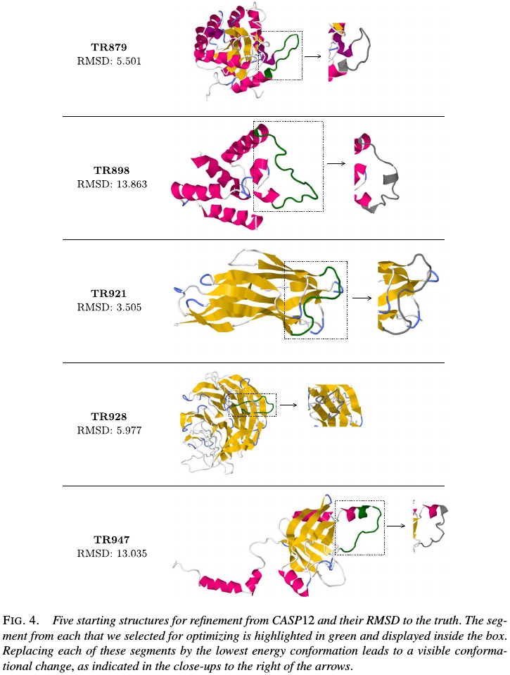
five examples from the CASP12 experiment in May-July2016, chosen to represent a wide range of accuracies in their given starting 3D structures. Select one segment from each for optimization using our method, on the 3D ribbon structures shown these are highlighted in green.

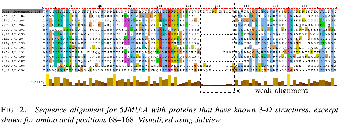
The true structure for the sequence with CASP ID TR879 was publicly released after CASP as 5JMU:A in the PDB. Use that example to describe how segments in the given structure might be selected for optimization without knowledge of the true structure.

1. generate a sequence alignment for the amino acid sequence of TR879, by running HHpred to search the PDB. It can be seen that the region ~123-134 has little or no alligment matches.
2. determine the secondary structure elements of the given 3D structure by running Dictionary of protein secondary structure (DSSP), this showed that the given starting structure has a coil region from positions 120-130 followed by an $\alpha$-helix beginning at position 131.
3. thus to cover most of that poor alignment region without breaking the long $\alpha$-helix in the given struture, chosen the segment 120-130 for energy-guided optimization.

Similarly, chose one segment to optimize from each of the five proteins, except TR898, for which no sequence alignments could be found and simply selected the long coil segment.

Apply the method to these segments, using $N=10,000$ particles and an RMSD cutoff of 0.25 Angstroms for pruning conformations that are too similar. For each segment output 5000 conformations, from which we selected the conformations with the lowest energy. For example, zoom into the region of interest and plot five sampled conformations with the lowest energy, and these five conformations are geometrically quite different from that of the given structure, and are also noticeably distinct geometrically among themselves. Their energy values are all within a fairly tight range ~246-266，which indicates that we are obtaining good coverage of distinct regions of the low-energy conformational space according to this energy function.

It can also be observed that the lowest energy conformation is not necessarily the best one according to this metric.

While RMSD is often computed on backbone atoms only, it can also be computed with side chain atoms as well (all-atom RMSD) to include an assessment of side chain accuracy. An alternative metric for measuring te similarity of two protein structures is the Global Distance Test (GDT)

Predict reconstructed loop segments

Testing the efficacy of the method in a controlled setting, where direct comparisons can be made with the ground truth. In the reconstruction problem, a segment is deleted from a true structure in the PDB, and a sampling method is tasked with generating conformations for the missing segment with the rest of the true structure held fixed.

Evaluate the method using 20 segments from a data set, which were selected specifically for study as examples of coil segments that connect $\alpha$-helices and $\beta$-sheets, that is known as loops in the bioinformatics literature, and hence this is known as the loop reconstruction problem. Most methods that have been proposed in the literature for loop reconstruction do not attempt to minimize energy as part of sampling. Make comparisons with the state-of-the-art DiSGro method.

The comparison is a useful test for the efficacy of the methodological innovations and in particular how the energies of the sampled conformations compare when evaluated according to the same energy function. DiSGro incorporates dihedral angle probabilities in an ad hoc manner to guide sampling, and then evaluates final conformations according to their pairwise distance energy function only.

Assessing different energy functions for sampling ad prediction

Assessing the accuracy of different energy functions for conformational sampling and prediction. For a given sequence or segment, the ideal energy function should assign the lowest energy values to conformations that are closet to the truth. Thus with an effective sampling method and the guidance of a good energy function, we ought to find low-energy conformations that should also be close to the truth.

energy models for atomic interactions:

• DiSGro energy function
• DFIRE, a statistical approximation of free energy
• the Lennard-Jones potential

Two evaluation metrics for each of the three energy functions:

• the smallest RMSD among the 5000 sampled conformations: assess how the energy function helps guide the construction of the particle population, in the sense of whether particles help guide the construction of the particle population, in the sense of whether particles with low RMSD to the truth can be retained under the model as particles propagate.
• the RMSD of the lowest energy function: assess how the energy function performs when selecting the lowest energy conformation as the prediction.