Bootstrap Hypothesis Testing
Posted on (Update: )
This report is motivated by comments under Larry’s post, Modern Two-Sample Tests.
Larry’s post
Consider two independent samples, $X_1,\ldots,X_n\sim P$ and $Y_1,\ldots,Y_m\sim Q$. To test $H_0:P=Q$ versus $H_1:P\neq Q$.
Larry highlighted the importance and amazement of Permutation Method and three innovated test statistics.
Kernel Tests
Firstly choose a kernel $K$, such as the Gaussian kernel,
\[K_h(x,y) = \exp\left(-\frac{\Vert x-y\Vert^2}{h^2}\right)\,.\]The test statistic is
\[T_h = \frac{1}{n^2}\sum_{i=1}^n\sum_{j=1}^nK_h(X_i,X_j) -\frac{2}{mn}\sum_{i=1}^n\sum_{j=1}^mK_h(X_i,Y_j)+\frac{1}{m^2}\sum_{i=1}^n\sum_{j=1}^nK_h(Y_i,Y_j)\,,\]where $K_h(x,y)$ can be seen as a measure of similarity between $x$ and $y$. To avoid the tunning parameter $h$, we can choose
\[T = \sup_{h\ge 0}T_h\,.\]Energy Test
Based on estimating the following distance between $P$ and $Q$:
\[D(P,Q)=2\E\Vert X-Y\Vert - \E\Vert X-X'\Vert -\E \Vert Y-Y'\Vert\]where $X,X’\sim P$ and $Y,Y’\sim Q$. The test statistic is a sample estimate of this distance.
The Cross-Match Test
Ignore the labels and put the data into non-overlapping pairs. Let $a_0$ be the number of pairs of type $(0,0)$, let $a_2$ be the number of pairs of type $(1,1)$, and let $a_1$ be the number of pairs of type $(0,1)$ and $(1,0)$.
Define
\[T=a_1.\]Confusion
After reading the great post, I continue to go through the comments, and one of Larry’s responses attracts me,
The permutation test is exact. The bootstrap is only approximate.
Although Larry had explained the above conclusion, such as,
It is exact no matter how many random permutations you use. Exact means: Pr(type I error ) <= alpha
The only assumptions are i.i.d. No stronger than usual
They are similar but not the same. The bootstrap samples n observations from the empirical distribution. (Actually, in a testing problem, the empirical has to be corrected to be consistent to the null hypothesis). The type I error goes to 0 as the sample size goes to infinity. In the permutation test, the type I error is less than alpha. No large sample approximation needed.
I also confused. So I resort to Google for help. Noa Haas’s slide helps me a lot, and find more formerly discussion in Efron and Tibshirani (1994).
Bootstrap Hypothesis Testing
Two sample test
Just in the setting of Larry’s post, we want to test $H_0:P=Q$ versus $H_1:P\neq Q$.
In the permutation test, the distribution under the null hypothesis $F_0$ is defined as the distribution of possible orderings of the labels, while Bootstrap uses a “plug-in” style estimate for $F_0$.
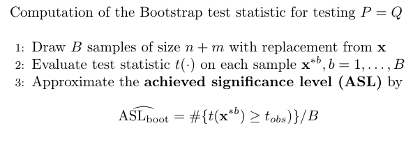
Quote Efron and Tibshirani (1994)’s discussion about the relationship between the permutation test and the bootstrap.
“A permutation test exploits special symmetry that exists under the null hypothesis to create a permutation distribution of the test statistic. For example, in the two-sample problem when testing $P=Q$, all permutations of the order statistic of the combined sample are equally probable. As a result of this symmetry, the ASL from a permutation test is exact: in the two-sample problem, $\mathrm{ASL}_{\mathrm{perm}}$ is the exact probability of obtaining a test statistic as extreme as the one observed, having fixed the data values of the combined sample.
“In contrast, the bootstrap explicitly estimates the probability mechanism under the null hypothesis, and then samples from it to estimate the ASL. The estimate $\widehat{\mathrm{ASL}}_{\mathrm{boot}}$ has no interpretation as an exact probability, but like all bootstrap estimates is only guaranteed to be accurate as the sample size goes to infinity. On the other hand, the bootstrap hypothesis test does not require the special symmetry that is needed for a permutation test, and so can be applied much more generally.
One sample test
Suppose we have sample $\x=(x_1,x_2,\ldots,x_n)$, and want to test $H_0:\mu= \mu_0$ against $\H_1:\mu\neq \mu_0$. In this case, we don’t have a symmetry, and hence the permutation test in unavailable. Suppose the test statistic is
\[t(\x) = \frac{\sqrt n(\bar x-\mu_0)}{\hat\sigma}\,.\]To perform Bootstrap hypothesis testing, we need a distribution that estimates the population of treatment times under $H_0$. Note first that the empirical distribution $\hat F$ is not an appropriate estimate for $F$ because it does not obey $H_0$. That is, the mean of $\hat F$ is not necessarily equal to $\mu_0$. A simple way is to translate the empirical distribution $\hat F$ so that it has the desired mean, i.e.,
\[\tilde x_i = x_i -\bar x+\mu_0\,.\]Then sample $\tilde x_1^*,\ldots,\tilde x_n^*$ with replacement from $\tilde x_1,\ldots,\tilde x_n$, and for each bootstrap sample compute the test statistic
\[t(\tilde \x^\*) = \frac{\sqrt n(\bar{\tilde x^\*}-\mu_0)}{\hat{\tilde\sigma^\*}}\]The first guide in Hall, P., & Wilson, S. R. (1991). Two Guidelines for Bootstrap Hypothesis Testing. Biometrics, 47(2), 757–762. JSTOR. is exactly related to this topics.
Simulation
Problem 16.4 of Efron and Tibshirani (1994).
Generate 100 samples of size 7 from a normal distribution with mean 129.0 and standard deviation 66.8. For each sample, perform a bootstrap hypothesis test by using the empirical distribution and the translated empirical distribution.
Compute the average of ASL for each test, averaged over the 100 simulations. And repeat with mean 170.
using StatsBase
using Distributions

# generate data
n = 7
μ = 129.0
σ = 66.8

# bootstrap test
function bootTest(data; B = 1000, trans::Bool = true)
    t = ones(B)
    x = copy(data)
    avg = mean(x)
    t_obs = sqrt(n) * (avg - μ) / sqrt(var(data))
    if trans
        x .= x .- avg .+ μ
    end
    for i = 1:B
        # sample
        idx = sample(1:n, n)
        x_star = x[idx]
        σ_star = sqrt(var(x_star))
        t[i] = sqrt(n) * (mean(x_star) - μ) / σ_star
    end
    return sum(t .> t_obs) / B
end
bootTest (generic function with 1 method)
function repx(mu, n = 100)
    p1 = ones(100)
    p2 = ones(100)
    for i = 1: 100
        P = Normal(mu, σ)
        x = rand(P, n)
        p1[i] = bootTest(x, trans = false)
        p2[i] = bootTest(x, trans = true)
    end
    return mean(p1), mean(p2)
end
repx (generic function with 2 methods)
If mu = 129.0, we should not reject the null hypothesis.
repx(μ)
(0.49734, 0.5011800000000001)
If mu = 170.0, the p-value should be much smaller than the previous one, and maybe we can reject the null hypothesis.
repx(170)
(0.58353, 0.16352)
Similarly, for the much larger mu, it is reasonable to reject $H_0$.
repx(300)
(0.6929299999999999, 0.00791)
It turns out that it is necessary to use the translated empirical distribution while performing bootstrap hypothesis testing, otherwise we would make mistakes.
Level-x parameters
Let $X_1, X_2, \ldots$ be a sequence of random variables with joint distribution $P$. Suppose that the data at hand can be modeled as a realization of the first $n$ random variables ${X_1,\ldots, X_n}\equiv \cX_n$. Also suppose that $\theta \equiv \theta(P)$ is a real-valued parameters of interest.
- level-1 parameter: parameters like $\theta$
Let $G_n$ denote the sampling distribution of the centered estimator $\hat\theta_n-\theta$. Then the mean square error of $\hat\theta_n$ is $\MSE(\hat\theta_n)=\int x^2dG_n(x)$.
- level-2 parameter: parameters like $\MSE(\hat\theta_n)$, which related to the sampling distribution of an estimator of a level-1 parameter
Bootstrap and other resampling methods can be regarded as general methods for finding estimators of level-2 parameters.
In the same vein,
- level-3 parameter: functionals related to the sampling distribution of an estimator of a level-2 parameter
- and so on
For such higher-level parameters, one may use a suitable number of iterations of the bootstrap or may successively apply a combination of more than one resampling method, e.g., Jackknife-After-Bootstrap method.
The general bootstrap principle:
- construct an estimator $\tilde F_n$ of $F$ from the available observations
- generate iid random variables from $\tilde F_n$
For dependent data, suppose that $X_1,X_2,\ldots$ is a sequence of stationary and weakly dependent random variables such that the series of the autocovariances of $X_i$’s converges absolutely. For simplicity, the parameter of interest is the population mean, i.e., $\theta=E(X_1)$. Consider the sample mean $\hat\theta_n=\bar X_n$ as an estimator of $\theta$, then the distribution of $\hat\theta_n-\theta$ depends not only on the marginal distribution of $X_1$, but it is a functional of the joint distribution of $X_1,\ldots,X_n$. For example,
\[\Var(\hat\theta_n) = n^{-1}[\Var(X_1) + 2\sum_{i=1}^{n-1}(1-i/n)\Cov(X_1,X_{i+1})]\]depends on the bivariate distribution of $X_1$ and $X_i$ for all $1\le i\le n$.
Note that since the process ${X_n}_{n\ge 1}$ is assumed to be weakly dependent, the main contribution to $\Var(\hat\theta_n)$ comes from the lower-order lag autocovariances.
As a consequence, accurate approximations for the level-2 parameter $\Var(\hat\theta_n)$ can be generated from the knowledge of the lag covariances $\Cov(X_1,X_{1+i}), 0\le i\le\ell$, which depend on the joint distribution of the shorter series ${X_1,\ldots,X_\ell}$ of the given sequence of observations ${X_1,\ldots,X_n}$.
For NBB, let $Y_1,\ldots, Y_b$ denote the $b$ blocks, defined by $Y_1={X_1,\ldots,X_\ell},\ldots,Y_b={X_{(b-1)\ell+1},\ldots,X_n}$. Note that because of stationarity, each block has the same ($\ell$-dimensional joint) distribution $P_\ell$. Furthermore, because of the weak dependence of the original sequence ${X_n}_{n\ge 1}$, these blocks are approximately independent for large values of $\ell$. Thus, $Y_1,\ldots, Y_b$ gives a collection of “approximately independent” and “identically distributed” random vectors with common distribution $P_\ell$.
Let $\cL(W; Q)$ denote the probability distribution of a random quantity $W$ under a probability measure $Q$. For the random quantity $T_n=t_n(\cX_n;\theta_n(P_n))$ of interest, the approximations involved in application of the bootstrap principle may be summerized by the following description:
\[\begin{align} \cL(T_n;P_n) &= P_n(t_n(\cX_n;\theta_n(P_n))\in \cdot)\\ &\approx P_\ell^b(t_n(\cX_n; \theta_n(P_\ell^b))\in \cdot)\\ &\approx \tilde P_\ell^b(t_n(\cX_n^\star; \theta_n(\tilde P_\ell^b))\in \cdot)\\ &= \cL(T_n^\star;\tilde P_\ell^b) \end{align}\]Block Bootstrap
- MBB: boundary effect as it assigns lesser weights to the observations toward the beginning and the end of the data set than to the middle part. For $\ell \le j \le n - \ell$, the $j$-th observation $X_j$ appears in exactly $\ell$ of the blocks, whereas for $1\le j\le \ell-1$, $X_j$ and $X_{n-j+1}$ appear only in $j$ blocks.
- NBB: a similar problem when $n$ is not a multiple of $\ell$.
References
- Efron B, Tibshirani RJ. An introduction to the bootstrap. CRC press; 1994 May 15.
- Lahiri, S. N. (2003). Resampling Methods for Dependent Data. Springer New York. https://doi.org/10.1007/978-1-4757-3803-2