A Bayesian Perspective of Deep Learning
Posted on
This note is for Polson, N. G., & Sokolov, V. (2017). Deep Learning: A Bayesian Perspective. Bayesian Analysis, 12(4), 1275–1304.
Abstract
Deep learning is a form of machine learning for nonlinear high dimensional pattern matching and prediction.
Traditional high-dimensional data reduction techniques are shallow learners:
- principal component analysis (PCA)
- partial least squares (PLS)
- reduced rank regression (RRR)
- projection pursuit regression (PPR)
Their deep learning counterparts exploit multiple deep layers of data reduction which provide predictive performance gains.
Stochastic gradient descent (SGD) training optimisation and Dropout (DO) regularization provide estimation and variable selection.
Bayesian regularization is central to finding weights and connections in networks to optimise the predictive bias-variance trade-off.
Introduction
The paper is Bayesian and probabilistic. They view the theoretical roots of DL in Kolmogorov’s representation of a multivariate response surface as a superposition of univariate activation functions applied to an affine transformation of the input variable. An affine transformation of a vector is a weighted sum of its elements (linear transformation) plus an offset constant (bias).
On the empirical side, they show that the advances in DL are due to
- new activation (a.k.a. link) functions, such as rectified linear unit (ReLU) instead of sigmoid function
- depth of the architecture and dropout as a variable selection procedure
- computationally efficient routines to train and evaluate the models as well as accelerated computing via graphics processing unit and tensor processing unit.
- deep learning has very well developed computational software where pure Markov Chain Monte Carlo (MCMC) is too slow.
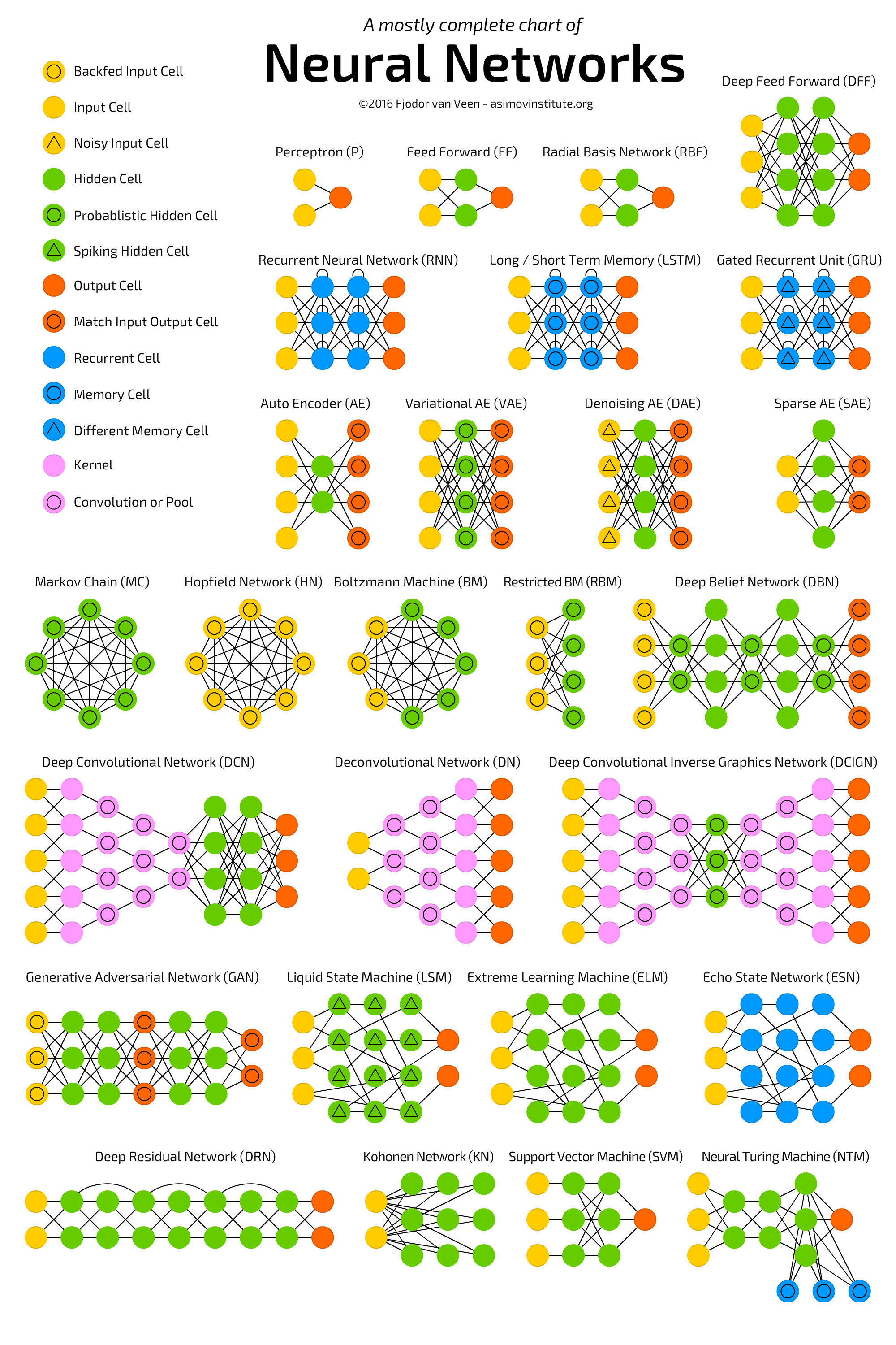
Most commonly used deep learning architectures are as follows (source):
Deep Probabilistic Learning
Given $\hat W,\hat b$, the negative log-likelihood defines $\cL$ as
\[\cL(Y,\hat Y)=-\log p(Y,Y^{\hat W,\hat b}(X))\,.\]To control the predictive bias-variance trade-off we add a regularization term and optimize
\[\cL_\lambda(Y,\hat Y)=-\log p(Y\mid Y^{\hat W,\hat b}(X)) - \log p(\phi(W,b)\mid \lambda)\]Deep predictors are regularized maximum a posterior (MAP) estimators, where
\[p(W,b\mid D)\propto p(Y\mid Y^{W,b}(X))p(W,b)\propto \exp\big(-\log p(Y\mid Y^{W,b}(X)-\log p(W,b))\big)\,.\]Training requires the solution of a highly nonlinear optimization
\[\hat Y:=Y^{\hat W,\hat b}(X)\quad\text{where}\quad (\hat W,\hat b):=\arg\,\max_{W,b}\log p(W,b\mid D)\,,\]and the log-posterior is optimised given the training data, $D=\{Y^{(i)},X^{(i)}\}_{i=1}^T$ with
\[-\log p(W,b\mid D)=\sum_{i=1}^T\cL(Y^{(i)},Y^{W,b}(X^{(i)})) + \lambda \phi(W,b)\,.\]Deep learning has the key property that $\Delta_{W,b}\log p(Y\mid Y^{W,b}(X))$ is computationally inexpensive to evaluate using tensor methods for very complicated architectures and fast implementation on large datasets.
For shallow architectures, the alternating direction method of multipliers (ADMM) is an efficient solution to the optimization problem.
Dropout for Model and Variance Selection
Dropout is a model selection technique designed to avoid over-fitting in the training process.
Suppose we wish to minimise $\MSE$, $\cL(Y,\hat Y)=\Vert Y-\hat Y\Vert_2^2$, then, when marginalizing over the randomness, we have a new objective
\[\arg\;\min_{W}\bbE_{D\sim \mathrm{Ber}(p)}\Vert Y-W(D*X)\Vert^2_2\,,\]where $*$ denotes the element-wise product. It is equivalent to, with $\Gamma = \sqrt{\diag(X^TX)}$,
\[\arg\;\min_W \Vert Y-pWX\Vert_2^2 + p(1-p)\Vert \Gamma W\Vert_2^2\,.\]Dropout then is simply Bayes ridge regression with a $g$-prior as an objective function. This reduces the likelihood of over-reliance on small sets of input data in training.
Dropout can also be viewed as the optimisation version of the traditional spike-and-slab prior, which has proven so popular in Bayesian model averaging.
Dropout also regularizes the choice of the number of hidden units in a layer.
Shallow Learners
Almost all shallow data reduction techniques can be viewed as consisting of a low dimensional auxiliary variable $Z$ and a prediction rule specified by a composition of functions
\[\hat Y = f_1^{W_1,b_1}(f_2(W_2X+b_2)) = f_1^{W_1,b_1}(Z)\,\quad \text{where }Z:= f_2(W_2X+b_2)\,.\]Stacked Auto-Encoders
Auto-encoding is an important data reduction technique. An auto-encoder is a deep learning architecture designed to replicate $X$ itself via a bottleneck structure. This means we select a model $F^{W,b}(X)$ which aims to concentrate the information required to recreate $X$.
Bayesian Inference for Deep Learning
History
- stochastic recurrent neural network (a.k.a. Boltzmann machines)
- accounting for uncertainty by integrating over parameters
- a general Bayesian framework for tuning network architecture and training parameters for feed forward architectures.
- Hamiltonian Monte Carlo (HMC) to sample from posterior distribution over the set of model parameters and then averaging outputs of multiple models.
- propose MCMC to jointly identify parameters of a feed forward neural network as well as the architecture.
Graphical models with deep learning encode a joint distribution via a product of conditional distributions and allow for computing (inference) many different probability distributions associated with the same set of variables.
The recent successful approaches to develop efficient Bayesian inference algorithms for deep learning networks are based on the reparameterization techniques for calculating Monte Carlo gradients while performing variational inference. Given the data $D=(X,Y)$, the variation inference relies on approximating the posterior $p(\theta\mid D)$ with a variation distribution $q(\theta\mid D,\phi)$, where $\theta=(W,b)$. The $q$ is found by minimizing the based on the Kullback-Leibler divergence between the approximate distribution and the posterior,
\[\KL(q\Vert p) = \int q(\theta\mid D,\phi)\log\frac{q(\theta\mid D,\phi)}{p(\theta\mid D)}d\theta\,.\]Replace minimization of $\KL(q\Vert p)$ with maximization of evidence lower bound (ELBO)
\[\ELBO(\phi) = \int q(\theta\mid D,\phi)\log \frac{p(Y\mid X,\theta)p(\theta)}{q(\theta\mid D,\phi)}\,.\]We have the relationship
\[\log p(D) = \ELBO(\phi) + \KL(q\Vert p)\,.\]The evidence lower bound name is follows from $\log p(D)\ge \ELBO(\phi)$.
To calculate the gradient, we can write ELBO as
\[\ELBO(\phi) = \int q(\theta\mid D,\phi)\log p(Y\mid X,\theta)d\theta - \int q(\theta\mid D,\phi)\log \frac{q(\theta\mid D,\phi)}{p(\theta)}d\theta\,.\]Two standards methods to calculate the gradient of the first term, $\nabla_\phi \E_q\log p(Y\mid X,\theta)$:
- use $\nabla_x f(x)=f(x)\nabla_x\log f(x)$: select $q(\theta\mid \phi)$ so that it is easy to compute its derivative and generate samples from it, the gradient can be efficiently calculated using Monte Carlo technique.
- use reparametrization by representing $\theta$ as a value of a deterministic function, $\theta=g(\epsilon,x,\phi)$, where $\epsilon\sim r(\epsilon)$ does not depend on $\phi$.
Finding Good Bayes Predictors
Adaptive Kernel predictors (a.k.a. smart conditional averager) are of the form
\[\hat Y(X) = \sum_{r=1}^RK_r(X_i,X)\hat Y_r(X)\,.\]Here $\hat Y_r(X)$ is a deep predictor with its own trained parameters.
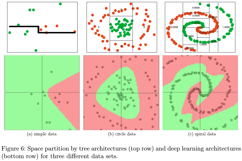
Deep learning can improve on traditional methods by performing a sequence of GLM-like transformations. Effectively DL learns a distributed partition of the input space.
The key difference between tree-based architecture and neural network based models is the way hyper-planes are combined.
A Bayesian probabilistic approach optimally weights predictors via model averaging with $\hat Y_k(x)=\E(Y\mid X_k)$
\[\hat Y(X) = \sum_{r=1}^Rw_k\hat Y_k(X)\,.\]Consider the Bayesian model of weak dependence, namely exchangeability. Suppose that we have $K$ exchangeable, $\bbE(\hat Y_i)=\bbE(\hat Y_{\pi(i)})$, and stacked predictors
\[\hat Y=(\hat Y_1,\ldots, \hat Y_K)\,.\]The randomized multiple predictor with equal weights provides the optimal Bayes predictive performance.
Algorithmic Issues
Stochastic Gradient Descent
SGD is a default gold standard for minimizing the a function $f(W,b)$ to find the deep learning weights and offsets. SGD simply minimizes the functions by taking a negative step along an estimate $g^k$ of the gradient $\nabla f(W^k,b^k)$ at iteration $k$.
The approximate gradient is estimated by calculating
\[g^k = \frac{1}{\vert E_k\vert}\sum_{i\in E_k}\nabla \cL_{w,b}(Y_i, \hat Y^k(X_i))\,,\]where $E_k\subset \{1,\ldots,T\}$ and $\vert E_k\vert$ is the number of elements in $E_k$.k
One caveat of SGD is that the descent in $f$ is not guaranteed, or it can be very slow at every iteration. Coordinate decent (CD), momentum-based modifications, and alternative directions method of multipliers (ADMM) can be alternatives.
The momentum-based versions of SGD, or so-called accelerated algorithms were originally proposed by Nesterov, so the name Nesterov’s momentum method (a.k.a. Nesterov acceleration).
Learning Shallow Predictors
The basic sliced inverse regression (SIR) model takes the form $Y=G(WX,\epsilon)$. To find $W$, first slice the feature matrix, then analyze the data’s covariance matrices and slice means of $X$, weighted by the size of slice.
Discussion
Deep learning is a high dimensional nonlinear data reduction scheme, generated probabilistically as a stacked generalized linear model (GLM). This sheds light on how to train a deep architecture using SGD. This is a first order gradient method for finding a posterior mode in a very high dimensional space.