Calculating Marginal likelihood
Posted on
Abstract
The marginal likelihood is the normalizing constant for the posterior density, obtained by integrating the product of the likelihood and the prior w.r.t. model parameters.
Study methods to quickly compute the marginal likelihood of a single fixed tree topology.
Benchmark the speed and accuracy of 19 different methods to compute the marginal likelihood of phylogenetic topologies on a suite of real datasets.
The results show that the accuracy of these methods varies widely, and that accuracy does not necessarily correlate with computational burden.
Introduction
Reasons to compute the marginal likelihood: The Bayesian inference allow the marginal likelihood to be avoided, but one potential application of these marginal likelihood computations is the development of fast, MCMC-free Bayesian phylogenetic inference.
One need to identify a large enough set of a posterior highly probable tree topologies, such as with a new optimization-based method called phylogenetic topographer (PT). Once a set of promising tree topologies is formed, we can compute their marginal likelihoods, then renormalize these marginal likelihoods (perhaps after multiplying by a prior) to obtain approximate posterior probabilities of tree topologies.
JC69 model: the simplest nucleotide substitution model
Methods
Consider a (fixed) unrooted topology $\tau$ for $S$ species with unconstrained branch length vector $\btheta = (\theta_1,\theta_2,\ldots,\theta_{2S-3})$ and the JC69 model, which assumes equal frequencies and equal substitution rate for all pairs of nucleotides.
\[p(\btheta\mid \tau, D) = \frac{p(D\mid \btheta, \tau)p(\btheta\mid \tau)}{\int p(D\mid \btheta, \tau)p(\btheta\mid \tau)d\btheta}\,.\]Typically, let $p(\btheta\mid\tau)=p(\btheta)=\prod p(\theta_i)$.
Two categories for calculating the marginal likelihood:
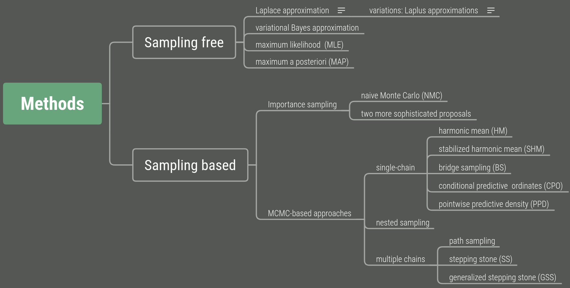
Variational inference
Transform posterior approximation into an optimization problem using a family of approximate densities. Aim to find the member of that family with the minimum Kullback-Leibler (KL) divergence to the posterior distribution of interest:
\[\bphi^* = \underset{\bphi\in \bPhi}{\arg\min} \KL(q(\btheta;\bphi)\Vert p(\btheta\mid D,\tau))\,,\]where $q(\btheta;\bphi)$ is the variational distribution.
Note that
\[\begin{aligned} \KL(q(\btheta;\bphi)\Vert p(\btheta\mid D,\tau)) &= \E[\log q(\btheta;\bphi)] - \E[\log p(\btheta\mid D,\tau)]\\ &= \E[\log q(\btheta;\bphi)]-\E[\log p(\btheta,D\mid \tau)] + \log p(D\mid\tau)\\ &=-\ELBO(\bphi) + \log p(D\mid\tau)\,, \end{aligned}\]where ELBO stands for the evidence lower bound. Then we can use the ELBO estimate
\[\hat p_\ELBO(D\mid\tau) := \max_{\bphi\in \bPhi}\ELBO(\bphi)\]to approximate the marginal likelihood of a topology.
Use a Gaussian variational mean-field approximation applied to log-transformed branch lengths to ensure that the variational distribution stays within the support of the posterior. Assume
\[q(\btheta;\bphi) = \prod q(\theta_i;\bphi_i)\]where $q(\theta_i;\bphi_i)$ is a log-normal density and $\bphi_i=(\mu_i,\sigma_i)$.
Benchmarks
Benchmark the 19 methods for estimating fixed-free marginal phylogenetic likelihood on 5 empirical datasets from a suite of standard test datasets.
Instead of focusing primarily on the accuracy of the estimate of the single-tree marginal likelihoods, the authors focus on the approximate posterior of topologies by applying the marginal methods to each and normalizing the result. Take measures of the goodness of these posteriors.
To compare marginal likelihood methods’ accuracy and precision, establish a ground truth for $p(\tau_i\mid D)$ for each tree topology $\tau_i$ by extensive runs.
Two different measures to determine closeness of an approximate posterior to the golden run posterior
- The root mean-squared deviation (RMSD) of the probabilities of splits: $\mathrm{RMSD}=\sqrt{\frac 1S\sum_i(\hat f(s_i)-f(s_i))^2}$, where $s_i$ is a split and $S$ the number of splits in the tree topology set, and \(\begin{aligned} f(s_i)&=\sum_jp(\tau_j\mid D)1_{s_i\in \tau_j}\\ \hat f(s_i)&=\sum_j\hat p(\tau_j\mid D)1_{s_i\in \tau_j} \end{aligned}\)
- KL divergence to assess how well the posterior probabilities of topologies are estimated: $\KL(\p\Vert \hat\p)$, where $\hat\p=(\hat p(\tau_1\mid D),\ldots,\hat p(\tau_N\mid D))$, $\p=(p(\tau_1\mid D),\ldots, p(\tau_N\mid D))$ and $N$ is the number of unique topologies in the $95\%$ posterior credible set of the golden run.
Future directions
- The paper restricted to fixed-topology inference under the simplest substitution model. Future work should generalize beyond this simplest model to obtain a marginal likelihood across all continuous model parameters for more complex models.
- Investigate the effect of modelling correlation between model parameters.
- Find some way to reduce the inter-dataset variability of the Laplus approximations.
- Develop novel bridge sampling to apply this method more broadly, not just for fixed topology model.
- Develop a diagnostic to determine an appropriate number of power posteriors that is required to accurately estimate marginal likelihoods.
- Integrating one of the fast or ultrafast methods with PT.
The program is available at GitHub: 4ment/physher and GitHub: 4ment/marginal-experiments.