The First Glimpse into Pseudolikelihood
Posted on
This post caught a glimpse of the pseudolikelihood.
As Wikipedia said, a pseudolikelihood is an approximation to the joint probability distribution of a collection of random variables.
Given a set of random variables, $X=X_1,\ldots,X_n$ and a set $E$ of dependencies between these random variables, where $\{X_i,X_j\}\not\in E$ implies $X_i$ is conditionally independent of $X_j$ given $X_i$’s neighbors, the pseudolikelihood of $X=x=(x_1,x_2,\ldots,x_n)$ is
\[\begin{equation} \Pr(X=x) = \prod_i\Pr(X_i=x_i\mid X_j=x_j\;\text{for all $j$ for which } \{X_i,X_j\}\in E)\,. \label{eq:pseudoll} \end{equation}\]In a word, the pseudolikelihood is the product of the variables, with each probability conditional on the rest of the data.
Murphy (2012) provides a motivation $\eqref{eq:pseudoll}$ base on MRFs.
Consider an MRF in log-linear form:
\[p(\y\mid \btheta) = \frac{1}{Z(\btheta)}\exp\Big(\sum_c\btheta_c^T\bphi_c(\y)\Big)\,,\]where $c$ indexes the cliques.
The objective for maximum likelihood is
\[\ell_{\mathrm{ML}}(\btheta) = \frac 1N \sum_i\log p(\y_i\mid\btheta)\]The derivative for the weights of a particular clique, $c$, is given by
\[\begin{align*} \frac{\partial \ell_{\mathrm{ML}}}{\partial \btheta_c} &= \frac 1N\Big[\bphi_c(\y_i)-\frac{\partial}{\partial \btheta_c}\log Z(\btheta)\Big]\\ &= \underbrace{\Big[\frac 1N \sum_i \bphi_c(\y_i)\Big]}_{\text{clamped terms}}-\underbrace{\bbE[\bphi_c(\y)\mid \btheta]}_{\text{unclamped term}}\\ &= \bbE_{p_{\mathrm{emp}}}[\bphi_c(\y)]-\bbE_{p(\cdot\mid\btheta)}[\bphi_c(\y)]\,. \end{align*}\]Let the gradient be zero, we will get moment matching:
\[\bbE_{p_{\mathrm{emp}}}[\bphi_c(\y)]=\bbE_{p(\cdot\mid\btheta)}[\bphi_c(\y)]\,.\]One alternative to MLE is to maximize the pseudo likelihood, defined as follows:
\[\ell_{\mathrm{PL}}(\btheta) = \frac 1N\sum_{i=1}^N\sum_{d=1}^D\log p(y_{id}\mid \y_{i,-d},\btheta)\,,\]which is also called the composite likelihood.
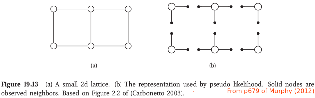
The PL approach can be illustrated by the following figure for a 2d grid. This objective is generally fast to compute since each full conditional $p(y_{id}\mid \y_{i,-d},\btheta)$ only requires summing over the states of a single node, $y_{id}$, in order to compute the local normalizing constant.
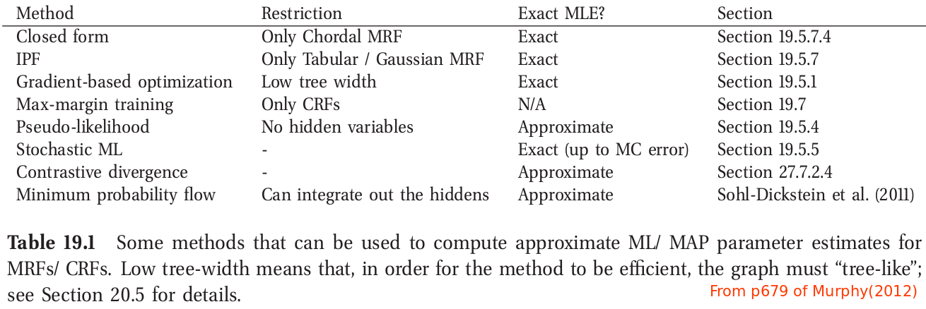
By the way, there are many methods to compute the MLE/MAP, as show in the following table.