The Kalman Filter and Extended Kalman Filter

Posted on Jan 21, 2019

Linear Dynamical System

In a linear dynamical system, the variation of a state vector, an $N$-dimensional vector denoted $\x$, equals to a constant matrix, $\A$, multiplied by $\x$. This variation can take two forms: either as a flow, in which $\x$ varies continuously with time

or as mapping, in which $\x$ varies in discrete steps,

Kalman Filter

The Kalman Filter are based on linear dynamical systems discretized in the time domain. They are modeled on a Markov chain built on linear operators perturbed by errors that may includes Gaussian noise. The state of the system is represented as a vector of real numbers.

At each discrete time increment,

• a linear operator is applied to the state to generate the new state, with some noise mixed in, and optimally some information from the controls on the system if they are known.
• another linear operator mixed with more noise generates the observed outputs from the true state.

Difference between Kalman Filter and HMM: The hidden state variables take values in a continuous space as opposed to a discrete state space as in the HMM.

The setting for the Kalman filter is the following linear state-space system. Given $x_0\sim N(\hat x_0,\Sigma_0)$, let

The Kalman filter provides recursive estimators for $x_t$:

where $\Sigma_t=\E(x_t-\hat x_t)(x_t-\hat x_t)’$, and $K_t$ is called the Kalman gain. The Kalman filter can be written in terms of the “observer system”:

where the random vector $a_t$ is called the innovation in $y_t$, being the part of $y_t$ that cannot be forecast linearly from its own past.

The formal derivation of the Kalman filter can be found in the appendix of Ljungqvist and Sargent (2004)

Example: Track Missile

This example is adopted from A First Look at the Kalman Filter.

Suppose we want to track a missile whose current location is $x\sim N(\hat x,\Sigma)$, where $\hat x=[0.2, -0.2]^T$ and

The sensor can report the location $y$ of the missile with some noise $v\sim N(0,R)$, so we have

where $G=I$ and $R=0.5\Sigma$.

The move of the missile can be interpreted as

where $A=\diag\{1.2,-0.2\}$ and $w\sim N(0,Q)$ where $Q=0.3\Sigma$.

Hence, we have the following setting up:

Σ = [0.4 0.3; 0.3 0.45]
x_hat = [0.2, -0.2]
G = Array(1.0I, 2, 2)
R = 0.5 .* Σ
A = [1.2 0
     0 -0.2]
Q = 0.3Σ

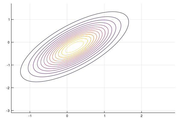
Firstly, we can illustrate our (prior) belief on the current position $x$ with contour map,

# plotting objects
x_grid = range(-1.5, 2.9, length = 100)
y_grid = range(-3.1, 1.7, length = 100)

# generate distribution
dist = MvNormal(x_hat, Σ)

# plot
contour(x_grid, y_grid, (x, y) -> pdf(dist, [x, y]), cbar = false)

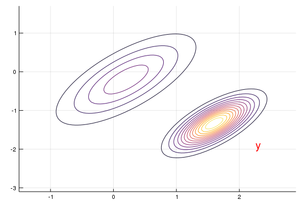
After obtaining the observation of the sensor, $y$, we can update our belief for the location via Bayes’ Theorem:

where

Remark: Here I derived the posterior distribution from scratch, but we can directly use the results of conjugate prior for convenience. And there is a good cheat sheet about Matrix Identities.

y = [2.3, -1.9]
annotate!(y[1], y[2], text("y", :red))

# define posterior objects
M = Σ * G' * inv(G * Σ * G' + R)
x_hat_F = x_hat + M * (y - G * x_hat)
Σ_F = Σ - M * G * Σ

newdist = MvNormal(x_hat_F, Symmetric(Σ_F))
contour!(x_grid, y_grid, (x, y)->pdf(newdist, [x, y]), cbar = false)

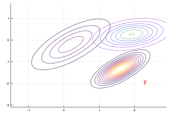
Finally, we can predict the next location by using the filtering distribution $p(x\mid y)\sim N(\hat x_f,\Sigma_f)$:

which is exactly $\eqref{eq:kf}$, where $K=\Sigma G’(R+G\Sigma G’)^{-1}$.

new_x_hat = A * x_hat_F
new_Σ = A * Σ_F * A' + Q
predictdist = MvNormal(new_x_hat, Symmetric(new_Σ))
contour!(x_grid, y_grid, (x, y)->pdf(predictdist, [x, y]), cbar = false, color = :lightrainbow)

Extended Kalman Filter

According to wikipedia, the EKF is the nonlinear version of the Kalman filter, which is the de facto standard in the theory of nonlinear state estimation, navigation systems and GPS.

In the extended Kalman filter, the state transition and observation models doesn’t need to be linear functions of the state but may instead be differentiable functions,

Use the simple but elegant trick–Taylor series of the first order–to linearize around a working point.

Example: Logistic growth

This example is adopted from Dominic Steinitz’s Fun with (Extended Kalman) Filters and Mage’s Extended Kalman filter example in R.

The logistic growth model can be written as a time-invariant dynamical system with growth rate $r$ and carrying capacity $k$:

which has the well known analytical solution:

We assume the growth rate $r$ is unknown and drawn from a normal distribution $N(\mu,\sigma^2)$ but the carrying capacity $k$ is known and we wish to estimate the growth rate by observing noisy value $y_i$ of the population at discrete times.

The state space and observation model can be written as:

Let $x_i\triangleq \begin{bmatrix} r_i & p_i\end{bmatrix}’$,

Here the state space model is purely deterministic, so there isn’t any evolution noise and hence $Q=0$. I use the following Julia code to implement this problem, which is inspired by Mage’s R code, but I think there might be some problems in Mage’s original code (see my comment in Mage’s blog for more details.)

# Inspired by https://magesblog.com/post/2015-01-13-extended-kalman-filter-example-in-r/

using Random, ForwardDiff
# parameters
k = 100
ΔΤ = 0.1
p0 = 0.1k
r = 0.2 

function logistG(r, p, k, t::Float64)
    return k * p * exp(r*t) / (k + p*(exp(r*t)-1) )
end

function logistG(r, p, k, t::Array{Float64})
    return k * p * exp.(r*t) ./ (k .+ p*(exp.(r*t).-1) )
end


# sample data 
Random.seed!(123);
obsVariance = 25
nObs = 250
v = randn(nObs) * sqrt(obsVariance)
p = logistG(r, p0, k, collect(1:nObs-1)*ΔΤ) 
p = insert!(p, 1, p0)
p = p + v

# estimate
res = ones(nObs, 2)

a(x::Vector) = [x[1], logistG(x[1], x[2], k, ΔΤ)]
G = [0 1]
# Evolution error
Q = zeros(2, 2)
# Observation error
R = obsVariance
# Prior
let
x = [r, p0]
Σ = [144.0 0;
     0 25.0]

for i = 1:nObs
    # Observation
    y = G * [r, p[i]]
    # Filter
    M = Σ * G' * 1/( (G * Σ * G')[1] + R)
    xf = x + M * (y - G * x)
    Σf = Σ - M * G * Σ

    A = ForwardDiff.jacobian(a, x)
    res[i,:] .= x
    # predict
    x = a(xf)
    Σ = A * Σf * A' + Q
end

end

# plot output
using Plots
time = collect(1:nObs) * ΔΤ
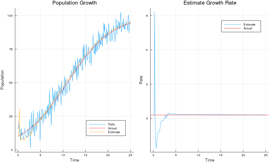
p1 = plot(time, p, legend = :bottomright, label = "Data", title = "Population Growth", xlab = "Time", ylab = "Population")
plot!(time, logistG(r, p0, k, time), color = :red, label = "Actual")
plot!(time, res[:,2], color = :orange, label = "Estimate")

p2 = plot(time, res[:,1], title = "Estimate Growth Rate", xlab = "Time", ylab = "Rate", label = "Estimate")
hline!([0.2], color = :red, label = "Actual")

plot(p1, p2, layout = (1,2), size=(1080, 640))

we can get the following result:

References

• L Ljungqvist and T J Sargent. Recursive Macroeconomic Theory. MIT Press, 2 edition, 2004.
• MAGE. Kalman filter example visualised with R. 2015.
• MAGE. Extended Kalman filter example in R
• Dominic Steinitz. Fun with (Extended Kalman) Filters. 2014.
• A First Look at the Kalman Filter