Conjugate Gradient for Regression
Posted on
The conjugate gradient method is an iterative method for solving a linear system of equations, so we can use conjugate method to estimate the parameters in (linear/ridge) regression.
Problem
Considering a linear system of equations
\[Ax=b\]where $A$ is a $n\times n$ symmetric positive definite matrix. It can be stated equivalently as the following minimization problem
\[\min\;\phi(x) =\frac{1}{2}x^TAx-b^Tx\]The gradient of $\phi$ equals the residual of the linear system,
\[\nabla \phi=Ax-b=r(x)\]so in particular at $x=x_k$ we have
\[r_k=Ax_k-b\]Conjugate Direction Method
A set of nonzero vectors ${p_0,p_1,\ldots,p_l}$ is said to be conjugate with respect to the symmetric definite matrix $A$ if
\[p_i^TAp_j=0\;\text{for all }i\neq j\]Given a starting point $x_0\in \IR^n$ and a set of conjugate directions ${p_0,p_1,\ldots,p_{n-1}}$, let us generate the sequence ${x_k}$ by
\[x_{k+1}=x_k+\alpha_kp_k\]where $\alpha_k$ is the one dimensional minimizer of the quadratic function $\phi(\cdot)$ along $x_k+\alpha p_k$, given explicitly by
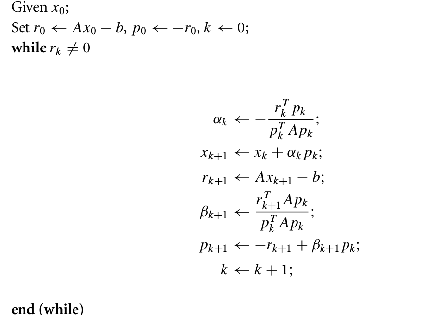
\[\alpha_k=-\frac{r_k^Tp_k}{p_k^TAp_k}\]Consider the function $\phi(\alpha)$ with respect step length $\alpha$
\(\phi(\alpha)=f(x_k+\alpha p_k)\) where $f(x) = \frac 12x^TAx-b^Tx$. Let $\phi’(\alpha)=0$, we have \(\alpha_k=-\frac{\nabla f_k^Tp_k}{p_k^TAp_k}\)
Conjugate Gradient Method
The conjugate gradient method is a conjugate direction method with a very special property: In generating its set of conjugate vectors, it can compute a new vector $p_k$ by using only the previous vector $p_{k-1}$
Each direction $p_k$ is chosen to be a linear combination of $-r_k$ and the previous direction $p_{k-1}$, that is
\[p_k=-r_k+\beta_kp_{k-1}\]where the scalar $\beta_k$ is to be determined by the requirement that $p_{k-1}$ and $p_k$ must be conjugate with respect to $A$. By premultiplying by $p_{k-1}^TA$ and imposing the condition $p_{k-1}^TAp_k=0$, we find that
\[\beta_k=\frac{r_k^TAp_{k-1}}{p_{k-1}^TAp_{k-1}}\]
Figure 1: CG-Preliminary Version
We can simplify $\alpha_k$ by using the property $r_k^Tp_{k-1}=0$ and obtain
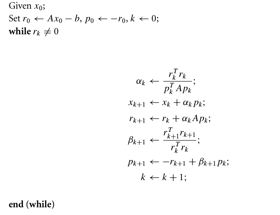
\[\alpha_k=\frac{r_k^Tr_k}{p_k^TAp_k}\]Also, we can simplify $\beta_k$ by using the property $r_{k+1}^Tr_k=0$ and obtain
\[\beta_{k+1}=\frac{r_{k+1}^Tr_{k+1}}{r_k^Tr_k}\]Then we obtain the following standard form of the conjugate gradient method

Figure 2: CG-Standard Version
Application in Regression
For linear regression, we can recognize $X’X$ as $A$ and $X’Y$ as $b$. It is cautious when there is multiple collinearity in $X$. Because $A$ should be a symmetric positive definite matrix, while $X’X$ doesn’t satisfy this requirement if there is multiple collinearity in $X$. Fortunately, for ridge regression, $X’X+\lambda I,\lambda>0$ is a symmetric positive definite matrix, so we don’t worry about multiple collinearity.
The following R code is for estimating the parameters in regression by using conjugate gradient method.
Simulation
Generate the dataset by random, and apply CG method to estimate the parameter of linear regression.
It is obvious that the differences of these two methods so small.
As for ridge regression, we can also test the performance by using the following R code.