Regularization-Free Principal Curves
Posted on
The note is for Gerber, S., & Whitaker, R. (2013). Regularization-Free Principal Curve Estimation. 18.
Abstract
The formal definition leads to some technical and practical difficulties. In particular, principal curves are saddle points of the mean-squared projection distance, which poses severe challenges for estimation and model selection.
The paper shows that the difficulties in model selection associated with the saddle point property of principal curves are intrinsically tied to the minimization of the mean-squared projection distance.
The paper introduces a new objective function, facilitated through a modification of the principal curve estimation approach, for which all critical points are principal curves and minima.
Regularization-Free Principal Curve Estimation
In manifold learning, the assumption is that a given sample is drawn from a low-dimensional manifold embedded in a higher dimensional space, possibly corrupted by noise.
Manifold learning refers to the task of uncovering the low-dimensional manifold given the high-dimensional observations. Several methods build directly on the manifold assumption and typically formulate the manifold estimation in terms of a graph embedding problem.
- Laplacian eigenmaps
- isomap
- locally linear embedding
The principal curve formulation casts manifold learning as a statistical fitting problem. Several approaches that fit a manifold model can be implicitly or explicitly related to the principal curve formulation.
- autoencoder neural networks
- self-organizing maps
- unsupervised kernel regression
While several methods have been proposed to estimate principal curves, a systematic approach to model selection remains an open question.
Without additional regularization, principal curve estimation results in space-filling curves, which have both lower training and test projection distance than curves that provide a more meaningful summary of the distribution.
Thus, all estimation approaches impose, implicit or explicit, regularity constraints on the curves.
The proposed formulation rests on the observation that minimizing $d(g, Y)^2$ allows principal curves $g$ to move away from saddle points and improve their fit by violating the self-consistency property.
Different from Hastie’s formulation to minimize $d(g, Y)^2 = \E[\Vert g(\lambda_g(Y))-Y\Vert^2]$, the paper fixes $g\equiv E[Y\mid \lambda(Y)]$ to the conditional expectation given $\lambda$ and let $\lambda$ be an arbitrary function $\lambda:\Omega\rightarrow \IR$. Call $\lambda$ the coordinate mapping and $E[Y\mid \lambda(Y)]$ the conditional expectation curve of $\lambda$.
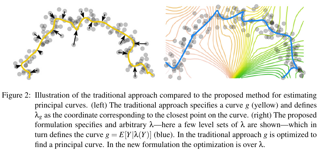
Now, the strategy is to optimize over the coordinate mapping $\lambda$ rather than $g$
Minimizing $d(\lambda, Y) = E[\Vert g(\lambda(Y))-Y\Vert^2]$ w.r.t. $\lambda$ leads to critical points that are, indeed, principal curves, but unfortunately they are still saddle points.
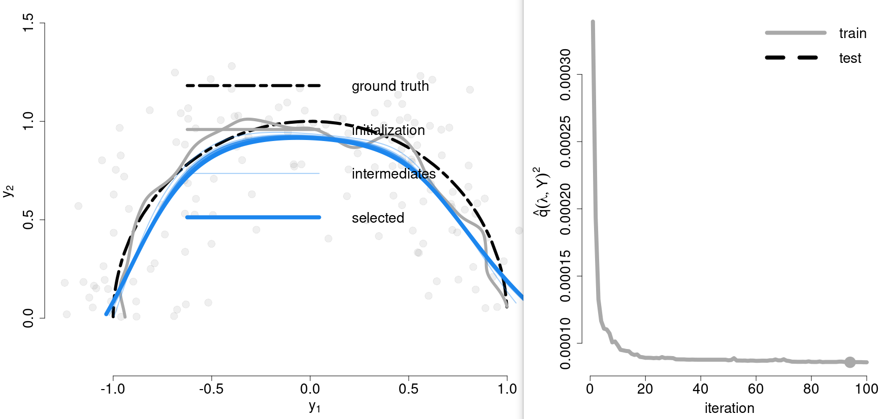
Then propose the following objective function, facilitated through the level-set based formulation, that penalizes nonorthogonality of the coordinate mapping $\lambda$
\[q(\lambda, Y)^2 = E\left[\langle g(\lambda(Y) -Y, \frac{d}{ds}g(s)\mid_{s=\lambda(Y)}\rangle^2\right]\]An algorithm for Data Sets
Gerber et al. (2009) proposed an algorithm to minimize $d(\lambda, Y)^2$ using a radial basis function expansion for $\lambda$ and a kernel regression for the conditional expectation $g$. For a data set $Y = {y_i}_1^n$, the radial basis function expansion is
\[\lambda(y) = \frac{\sum_{j=1}^nK(y-y_j)z_j}{\sum_{j=1}^nK(y-y_j)}\]with $K$ a Gaussian kernel with bandwidth $\sigma_\lambda$ and $Z={z_i}_1^n\in\IR$ a set of parameters.
The algorithm has been implemented in r-package cems. Currently, the package is not available on CRAN, so manually install it
install.packages("vegan")
install.packages("/media/weiya/PSSD/Downloads/cems_0.4.tar.gz", repos = NULL, type = "source")
then run the example,
cem.example.arc()