A pHMM Algorithm for Correcting Long Reads
Posted on (Update: )
second or third generation sequencing platforms: trade-offs between accuracy and read length
to get long and accurate reads: combine both technologies and the errorneous long reads are corrected using the short reads
- current approaches rely on various graph or alignment based techniques and do not take the error profile of the underlying technology into account.
- ? efficient machine learning algorithms that address these shortcomings have the potential to achieve more accurate integration of these two technologies
The paper proposed Hercules, the first (?) machine learning-based long read error correction algorithm.
- it models every long read as a profile HMM w.r.t. the underlying platform’s error profile.
- it learns a posterior transition/emission probability distribution for each long read to correct errors in these reads
Introduction
High Throughput Sequencing (HTS) technologies suffer from two fundamental limitations
- no platform is yet able to generate a chromosome-long read. Average read length ranges from 100bp to 20kb depending on the platform.
- reads are not error-free.
A base pair (bp) is a fundamental unit of double-stranded nucleic acids consisting of two nucleobases bound to each other by hydrogen bonds.
- Illumina: the most ubiquitous platform. produces the most accurate (~0.1% error rate), yet the shortest (100-150bp) reads.
- Pacific Biosciences Single Molecule, Real-Time (SMRT) sequencing technology is capable of producing > 10kb-long reads on average, though with a substantially higher (~15%) error rate
- Oxford Nanopore Technologies (ONT) platform: can generate longer reads (up to ~900kb), but their error rate is also higher (>15%)
The strengths and weaknesses of the platforms makes it attractive to combine them.
Two major categories for hybrid error correction methods
- align short reads onto long reads generated from the same sample, implemented by several tools. These algorithms fix the errors in long reads by calculating a consensus of the short reads over the same segment of the nucleic acid sequence.
- drawback: alignment based approaches are highly dependent on the performance of the aligner. Hence, accuracy, run time, and memory usage of the aligner will directly affect the performance of the downstream correction tool.
- align long reads over a de Bruijn graph constructed using short reads, and the $k$-mers on the de Bruijn graph that are connected with a long read are then merged into a new, corrected form of the long read.
- drawback: the resulting graph may contain bulges and tips, that are typically treated as errors and removed. Accurate removal of such graph elements relies on the availability of high coverage data to be able to confidently discriminate real edges from the ones caused by erroneous $k$-mers.
Herclues models each long and erroneous read as a template profile HMM. It uses short reads as observations to train the model via forward-backward algorithm, and learns posterior transition and emission probabilities. Finally, Hercules decodes the most probable sequence for each profile HMM using Viterbi algorithm.
main advantages of Hercules:
- reduce dependency on aligner performance
- alignment-based methods are dependent on the aligner’s full CIGAR string for each basepair to correct. They perform majority voting to resolve discrepancies among short reads with the assumption that all error types are equally likely to happen during correction.
- Hercules uses the starting positions obtained from an aligner, it does not depend on any other information provided by the aligner. It sequentially and probabilistically accounts for the evidence provided per short read, instead of just independently using majority voting per base-pair.
- directly incorporate experimentally observed error profiles of long reads that can be updated when the underlying sequencing technology improves, or adapted to new long read sequencing platforms.
Methods
Hercules correct errors (insertions, deletions, and substitutions) present in long read sequencing platforms such as PacBio SMRT and Oxford Nanopore Technologies, using reads from a more accurate orthogonal sequencing platform, such as Illumina.
Preprocessing
skip
pHMM structure
Goal: calculate the most likely (consensus) sequence the model would produce, among all possible sequences that can be produced using the letters in the alphabet $\Sigma$.
Overview of HMM
Three fundamental problems:
- Problem I (Likelihood): Given an HMM $\lambda = (\pi, A, B)$ and an observation sequence $O$, determine the likelihood $P(O\mid \lambda)$
- Problem II (Decoding): Given an observation sequence $O$ and an HMM $\lambda = (\pi, A, B)$, discover the best hidden state sequence $Q$
- Problem III (Learning): Given an observation sequence $O$ and the set of states in the HMM, learn the HMM parameters
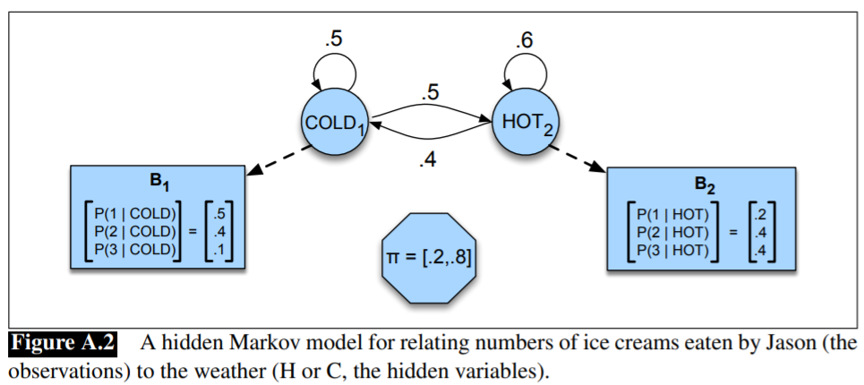
HMM for the ice cream task:
Problem III
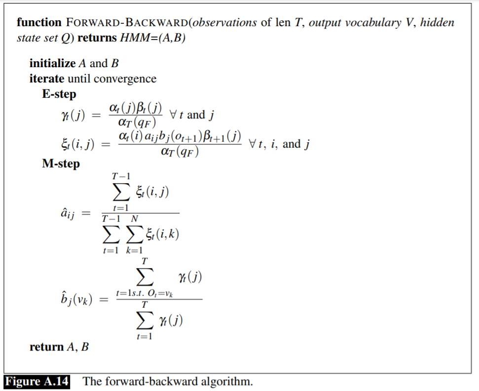
The standard algorithm is the forward-backward, or Baum-Welch algorithm, a special case of the EM algorithm.
First consider the much simpler case of training a fully visible Markov model, both the temperature and the ice cream count for every day are known. For example,
| 3 | 3 | 2 | 1 | 1 | 2 | 1 | 2 | 3 | ||
|---|---|---|---|---|---|---|---|---|---|---|
| hot | hot | cold | cold | cold | cold | cold | hot | hot |
Then the HMM parameters are just by maximum likelihood estimation from the training data.
First, we can compute $\pi$ from the count of the 3 initial hidden states:
\[\pi_h = 1/3, \pi_c = 2/3\,.\]Next, we can directly compute the $A$ matrix from the transitions, ignoring the final hidden states:
\[p(h\mid h)=\frac{2}{2+1}, p(c\mid h) = \frac{1}{2+1};\; p(c\mid c) = \frac{2}{2+1}, p(h\mid c) = \frac{1}{2+1}\,,\]and the $B$ matrix
\[p(1\mid h) = 1/4, p(2\mid h) = 1/4, p(3\mid h) = 3/4;\; p(1\mid c) = 3/5, p(2\mid c)=2/5, p(3\mid c)=0\,.\]For a real HMM, we cannot compute these counts directly from an observation sequence since we do not know which path of states was taken through the machine for a given input.
The backward probability $\beta$ is the probability of seeing the observations from time $t+1$ to the end, given that we are in state $i$ at time $t$
\[\beta_t(i) = P(o_{t+1}, o_{t+2},\ldots, o_T\mid q_t=i,\lambda)\]- initialization: $\beta_T(i)=1,1\le i\le N$
- recursion: $\beta_t(i) = \sum_{j=1}^Na_{ij}b_j(o_{t+1})\beta_{t+1}(j)$
- termination: $P(O\mid \lambda) = \sum_{j=1}^N\pi_jb_j(o_1)\beta_1(j)$
Assume we had some estimate of the probability that a given transition $i\rightarrow j$ was taken at a particular point in time $t$ in the observation sequence. If we knew this probability for each particular time $t$, we could sum over all times $t$ to estimate the total count for the transition $i\rightarrow j$.
Define the probability $\xi_t$ as the probability of being in state $i$ at time $t$ and state $j$ at time $t+1$, given the observation sequence and of course the model:
\[\xi(i, j) = P(q_t=i,q_{t+1}=j\mid O,\lambda)\]First, compute
\[P(q_t=i,q_{t+1}=j,O\mid\lambda)= \alpha_t(i)a_{ij}b_j(o_{t+1})\beta_{t+1}(j)\]and note that
\[P(O\mid \lambda)=\sum_{j=1}^N \alpha_t(j)\beta_t(j)\]Thus,
\[\xi_t(i, j) = \frac{\alpha_t(i)a_{ij}b_j(o_{t+1})\beta_{t+1}(j)}{\sum_{j=1}^N \alpha_t(j)\beta_t(j)}\]Thus,
\[\hat a_{ij} = \frac{\sum_{t=1}^{T-1}\xi_t(i, j)}{\sum_{t=1}^{T-1}\sum_{k=1}^N\xi_t(i, k)}\]Similarly,
\[\hat b_j(v_k) = \frac{\sum_{t=1, s.t. O_t=v_k}^T\gamma_t(j)}{\sum_{t=1}^T\gamma_t(j)}\,,\]where
\[\gamma_t(j) = \frac{\alpha_t(j)\beta_t(j)}{P(O\mid \lambda)}\,.\]