Multivariate Adaptive Regression Splines
Posted on
This note is for Friedman, J. H. (1991). Multivariate Adaptive Regression Splines. The Annals of Statistics, 19(1), 1–67.
MARS takes the form of an expansion in product spline basis functions, where the number of basis functions as well as the parameters associated with each one (product degree and knot selections) are automatically determined by the data.
This procedure is motivated by the recursive partitioning approach to regression and shares its attractive properties, but
- it produces continuous models with continuous derivatives
- it has more power and flexibility to model relationships that are nearly additive or involve interactions in at most a few variables
- it can be represented in a form that separately identifies the additive contributions and those associated with the different multivariate interactions.
Goal: model the dependence of a response variable $y$ on one or more predictor variables $x_1,\ldots,x_n$ given realizations (data) ${y_i,x_{1i},\ldots,x_{ni}}_1^N$. Suppose the data is generated from
\[y = f(x_1,\ldots,x_n) + \varepsilon\,,\]over some domain $(x_1,\ldots,x_n)\in D\subset \IR^n$, then the aim of regression analysis is to use the data to construct a function $\hat f$ that can serve as a reasonable approximation to $f(x_1,\ldots,x_n)$ over the domain $D$ of interest.
Lack of accuracy is often defined by the integral error
\[I = \int_D w(\bfx)\Delta[\hat f(\bfx), f(\bfx)]dx\,,\]or the expected error
\[E = \frac 1N\sum_{i=1}^Nw(\bfx_i)\Delta[\hat f(\bfx_i), f(\bfx_i)]\,,\]where $\bfx = (x_1,\ldots,x_n)$.
If future joint covariate values $\bfx$ can only be realized at the design points, then $E$ is appropriate; otherwise $I$ is more relevant.
Existing methodology
Global parametric modeling
Fit a parametric function $g(\bfx \mid {a_j}_1^p)$, and the coefficient is estimated by
\[\{a_j\}_1^p = \argmin \sum_{i=1}^N\left[y_i-g(\bfx\mid \{a_j\}_1^p)\right]^2\,.\]pros:
- requiring relatively few data points, and hence easy to interpret and rapidly computable.
cons:
- limited flexibility
- likely to produce accurate approximations only when the form of the true underlying function $f(\bfx)$ is close to the prespecified parametric one.
Nonparametric modeling
In low dimensional settings, global parametric modeling has been successfully generalized using three (related) paradigms
- piecewise parametric fitting: such as splines
- local parametric fitting
- roughness penalty methods
Low dimensional expansions
The ability of the nonparametric methods to often adequately approximate functions of a low dimensional argument, coupled with their corresponding inability in higher dimensions, has motivated approximations that take the form of expansions in low dimensional functions
\[\hat f(\bfx) = \sum_{j=1}^J \hat g_j(\bfz_j)\,,\]where each $\bfz_j$ is comprised of a small (different) preselected subset of ${x_1,\ldots,x_n}$.
Adaptive computation
An adaptive computation is one that dynamically adjusts its strategy to take into account the behavior of the particular problem to be solved, for example, the behavior of the function to be approximated.
In statistics, adaptive algorithms for function approximation have been developed based on two paradigms,
- recursive partitioning
- projection pursuit
projection pursuit
it uses an approximation of the form
\[\hat f(\bfx) = \sum_{m=1}^M f_m\left(\sum_{i=1}^n\alpha_{im}x_i\right)\,,\]that is, additive functions of linear combinations of the variables.
The univariate function $f_m$ ans the corresponding coefficients of the linear combinations appearing in their arguments, are jointly optimized to produce a good fit to the data based on some distance criterion.
Pros:
- even for small to moderate $M$, many classes of functions can be closely fit by approximations of this form.
- affine equivariance: the solution is invariant under any nonsingular affine transformation (rotation and scaling) of the original explanatory variables.
- it has some interpretive value (for small $M$) in that one can inspect the solution functions $f_m$ and the corresponding loadings in the linear combination vectors.
- evaluation of the resulting approximation is computationarlly fast
cons:
- there exist some simple functions that require large $M$ for good approximation
- it is difficult to separate the additive from the interaction effects associated with the variable dependencies (??)
- interpretation is difficult for large $M$
- the approximation is computationally time consuming to construct.
Recursive partition regression
It takes the form
\[\text{if }\bfx\in R_m\,,\quad \text{then }\hat f(\bfx) = g_m(\bfx \mid \{a_j\}_1^p)\,,\]where ${R_m}_1^M$ are disjoint subregions and the most common for $g_m$ is a constant function.
Pros:
- fairly rapid to construct and especially rapid to evaluate
Cons: some fairly severe restrictions that limit its effectiveness
- the approximating function is discontinuous at the subregion boundaries. It severely limits the accuracy of the approximation, especially when the true underlying function is continuous.
- certain typesof simple functions are difficult to approximate, such as linear functions
- it has difficulty when the dominant interactions involve a small fraction of the total number of variables
- one cannot discern from the representation of the model whether the approximating function is close to a simple one, such as linear or additive, or whether it involves complex interactions among the variables.
Adaptive regression splines
Recursive partitioning regression revisited
Replace the geometrical concepts of regions and splitting with the arithmetic notions of adding and multiplying.
The expansion is
\[\hat f(\bfx) = \sum_{m=1}^M a_mB_m(\bfx)\,,\]where the basis functions $B_m$ take the form
\[B_m(\bfx) = I(\bfx\in R_m)\,.\]Let $H[\eta]$ be a step function indicating a positive argument
\[H[\eta] = \begin{cases} 1 & \text{if $\eta\ge 0$}\\ 0 & \text{otherwise} \end{cases}\] \[\newcommand\LOF{\mathrm{LOF}}\]and let $LOF(g)$ be a procedure that computes the lack-of-fit of a function $g(\bfx)$ to the data.
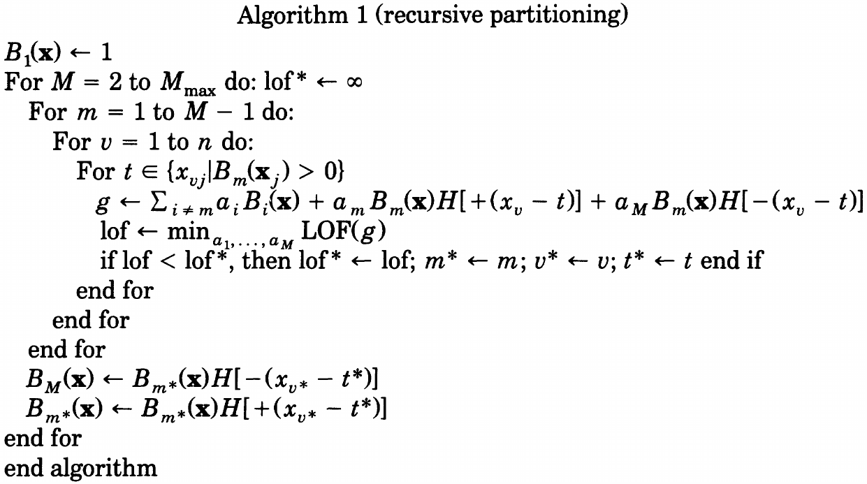
The basis functions produced by Algorithm 1 have the form
\[B_m(\bfx) = \prod_{k=1}^{K_m}H[s_{km}\cdot(x_{v(k,m)}-t_{km})]\]Continuity
The only aspect of Algorithm 1 that introduces discontinuity into the model is the use of the step function $H[\eta]$ as its central ingredient.
The choice for a continuous function to replace the step function is guided by the fact that the step function as used in Algorithm 1 is a special case of a spline basis function.
The one-sided truncated power basis functions for representing $q$-th degrees_the original used order should be corrected_{:.comment} splines are
\[b_q(x-t) = (x-t)_ +^q\]A two-sided truncated power basis is a mixture of functions of the form,
\[b_q^\pm (x-t) = [\pm(x-t)]_ +^q\]The step functions can be seen to be two-sided truncated power basis functions for $q=0$ splines.
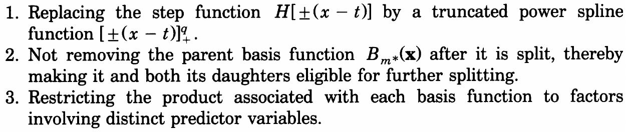
If we replace the step function by a $q > 0$ truncated power spline basis function, then these multivariate spline basis functions take the form
\[B_m^{(q)}(\bfx) = \prod_{k=1}^K\left[s_{km}(x_{v(k,m)}-t_{km})\right]_ +^q\,,\]but the resulting basis will not reduce to a set of tensor product spline basis functions.
The final basis functions can each have several factors can each have several factors involving the same variable in their product. Products of univariate spline functions on the same variable do not give rise to a spline function of the same order, except for the special case of $q=0$.
Permitting repeated (nested) splits on the same variable is an essential aspect contributing to the power of recursive partitioning.
A further generalization
The central operation in Algorithm 1 is to delete an existing (parent) basis function and replace it by both its product with a univariate truncated power spline basis function and the corresponding reflected truncated power function. The proposed modification involves simply not removing the parent basis function, i.e., the number of basis functions increases by two as a result of each iteration of the outer loop. All basis functions (parent and daughters) are eligible for further splitting.
This strategy also resolves the dilemma in the last section.
In summary, the modifications are
MARS
With the above modification, and consider $q=1$, we obtain the following MARS algorithm,
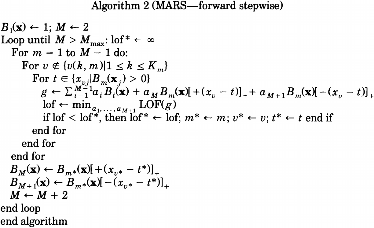
Unlike recursive partitioning, the corresponding regions are not disjoint but overlap, and hence removing a basis function does not produce a hole. A usual backward procedure can be applied,
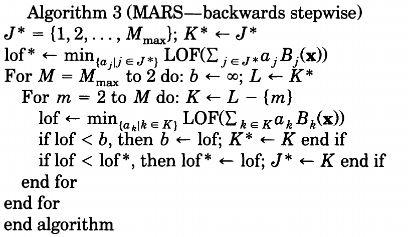
ANOVA decomposition
The result of applying Algorithm 2 and 3 is a model of the form,
\[\hat f(\bfx) = a_0 + \sum_{m=1}^Ma_m\prod_{k=1}^{K_m}[s_{km}(x_{v(k,m)}-t_{km})]_ +\]which can be recast into
\[\hat f(\bfx) = a_0 + \sum_{K_m=1}f_i(x_i) + \sum_{K_m=2}f_{ij}(x_i,x_j) + \sum_{K_m=3}f_{ijk}(x_i,x_j,x_k) + \cdots\]Model Selection
The GCV criterion is the average-squared residual of the fit to the data (numerator) times a penalty (inverse denominator) to account for the increased variance associated with increasing model complexity.
A cost complexity function is proposed to be
\[\tilde C(M) = C(M) + d\cdot M\,,\]where
\[C(M) = 1 + \trace(B(B^TB)^{-1}B^T)\]and the quantity $d$ represents a cost for each basis function optimization and is a (smoothing) parameter of the procedure (!!). Larger values for $d$ will lead to fewer knots being placed and thereby smoother function estimates.
- Friedman and Silverman (1989): take $d=2$ for $K_m=1$
One method for choosing a value for $d$ in any given situation would be to simply regard it as a parameter of the procedure that can be used to control the degree of smoothness imposed on the solution. Their simulations suggest that
- the optimal cost complexity function $\tilde C(M)$ to be used in the GCV criterion is a monotonically increasing function with decreasing slope as $M$ increases.
- $d=3$ is fairly effective, if somewhat crude
- the best value for $d$ is in the range $2\le d\le 4$.
- the actual accuracy in terms of either integral $I$ or expected $E$ is fairly insensitive to the value of $d$ in this range
- the value of the GCV criterion for the final MARS model does exhibit a moderate dependence on the value chosen for $d$
Degrees-of-continuity
the difficulty with higher order regression splines centers on so called end effects.
the strategy for producing a model with continuous derivatives is to replace the function
\[b(x\mid s, t) = [s(x-t)]_ +\]with a corresponding truncated cubic function of the form
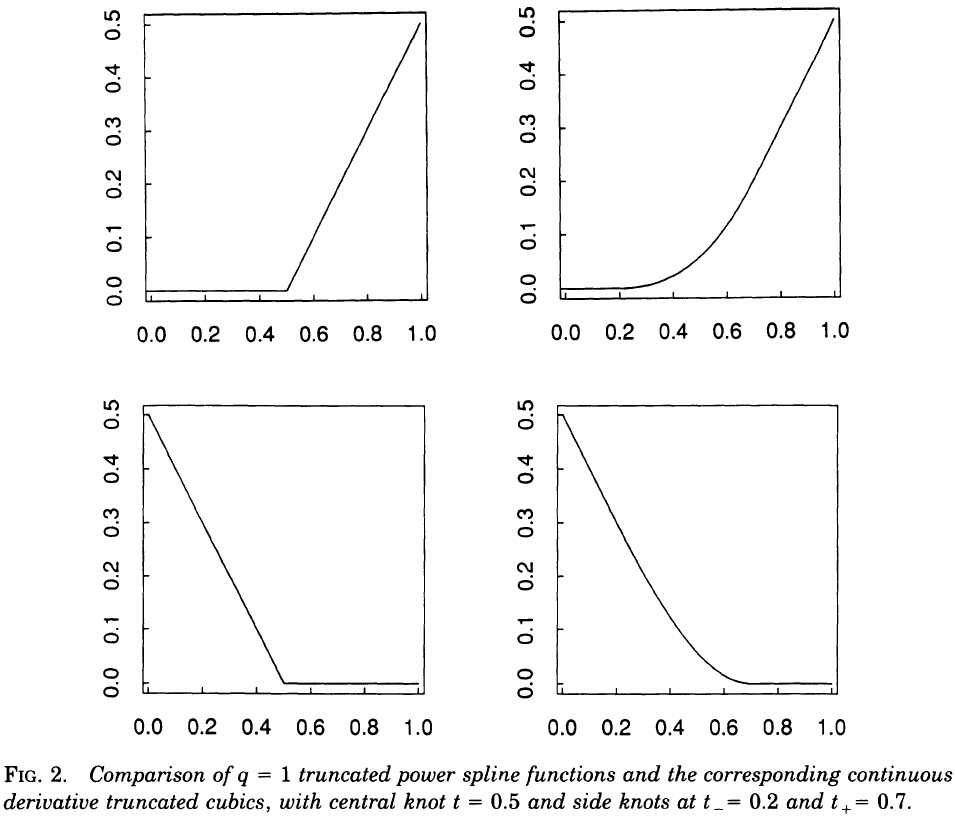
Knot optimization
skip…
Computational considerations
skip…
Simulations
the goal is to try to gain some understanding of its properties and to learn in what situations one might expect it to provide better performance than existing methodology.
Remarks
Constraints
one can
- limit the maximum interaction order
- limit the specific variables that can participate in interactions
Semiparametric modeling
\[\hat f_{sp}(\bfx) = \sum_{j=1}^Jc_jg_j(\bfx) + \hat f(\bfx)\,,\]where $\hat f(\bfx)$ takes the form of the MARS approximation, and $g_j(\bfx)$ are provided by user.
Collinarity
The problem is even more serious for (interactive) MARS modeling than for additive or linear modeling.
- it is difficult to isolate the separate contributions of highly collinear predictor variables to the functional dependence
- it is also difficult to separate the additive and interactive contributions among them.
Robustness
Since MARS uses a model selection criterion based on squared-error loss, it is not robust against outlying response values.
Use robust/resistant linear regression methods would provide resistance to outliers. The only advantage to squared-error loss in the MARS context is computational.
Conclusion
Aim of MARS: combine recursive partitioning and spline fitting in a way that best retains the positive aspects of both, while being less vulnerable to their unfavorable properties.