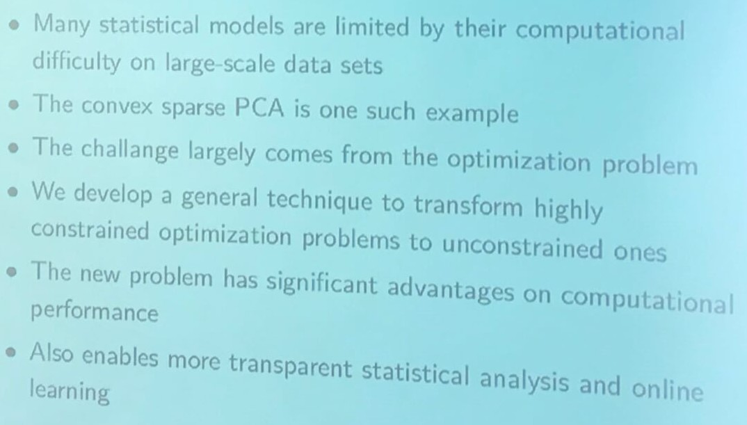
Gradient-based Sparse Principal Component Analysis
Posted on (Update: )
This post is based on the talk, Gradient-based Sparse Principal Component Analysis, given by Dr. Yixuan Qiu at the Department of Statistics and Data Science, Southern University of Science and Technology on Jan. 05, 2020.
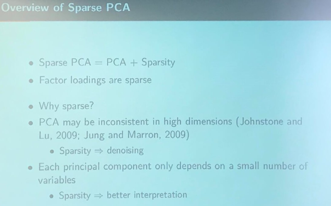
Overview of Sparse PCA
An Illustrative Example
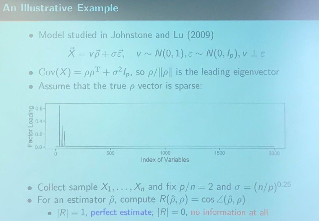
The reason why he chose $\sigma = (n/p)^{0.25}$ is that Johnstone and Lu (2009) claims
$\hat\brho$ is a consistent estimator of $\brho$ iff $p/n\rightarrow 0$. On the other hand, if
\[\lim\frac pn \frac{\sigma^4}{\Vert \brho\Vert^4} \ge 1\,,\]then $\lim_n R^2(\hat\brho,\brho) = 0$, i.e., $\hat\brho$ and $\brho$ are asymptotically orthogonal.
so the above slide should means that $\brho$ has been normalized.
PCA in High Dimensions $(p = 1000)$
I implement the toy example as follows:
library(elasticnet)
library(lattice)

# generate the data
sim.data <- function(p) {
  n = p / 2
  sigma = (1 / 2)^0.25
  # true rho
  rho.nonzero = c(0.6, 0.5, 0.2)
  rho = numeric(p)
  rho[sample(1:p, 3)] = rho.nonzero / sqrt(sum(rho.nonzero^2))
  Xmat = matrix(0, nrow = n, ncol = p)
  for (i in 1:n){
    Xmat[i, ] = rnorm(1) * rho + sigma * rnorm(p)
  }
  return(list(X = Xmat, rho = rho))
}

costheta <- function(x, y){
  sum(x * y) / sqrt(sum(x^2) * sum(y^2))
}
cpr.methods <- function(p) {
  data = sim.data(p)
  X = data$X
  rho = data$rho

  spca.hastie.varnum = elasticnet::spca(X, 1, 3, sparse = "varnum")$loadings
  spca.hastie.penalty10 = elasticnet::spca(X, 1, 10)$loadings
  spca.hastie.penalty100 = elasticnet::spca(X, 1, 100)$loadings
  spca.hastie.penalty1000 = elasticnet::spca(X, 1, 1000)$loadings
  pca = svd(X)$v[, 1]

  df = data.frame(1:length(rho),
                  rho,
                  pca,
                  spca.hastie.varnum,
                  spca.hastie.penalty10,
                  spca.hastie.penalty100,
                  spca.hastie.penalty1000)
  colnames(df) = c("idx",
                   "Truth",
                   paste0("PCA: ", costheta(rho, pca)),
                   paste0("Hastie's SPCA (varnum = 3): ", costheta(rho, spca.hastie.varnum)),
                   paste0("Hastie's SPCA (penalty = 10): ", costheta(rho, spca.hastie.penalty10)),
                   paste0("Hastie's SPCA (penalty = 100): ", costheta(rho, spca.hastie.penalty100)),
                   paste0("Hastie's SPCA (penalty = 1000): ", costheta(rho, spca.hastie.penalty1000)))
  return(df)
}
df = cpr.methods(1000)
xyplot(value~idx|variable, data = melt(df, id.vars = "idx"), type = "l",
       layout = c(1, 6),
       index.cond = list(c(6,5,4,3,2,1)),
       xlab = "Index",
       ylab = "Eigenvector")
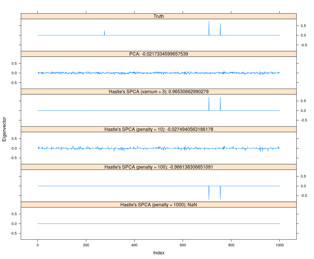
Here, I adopt Zou and Hastie’s elasticnet for Sparse PCA. Actually, Johnstone and Lu (2009) provided their MATLAB program, and there are some alternatives of sparse PCA, such as Erichson et al.’s SPCA.
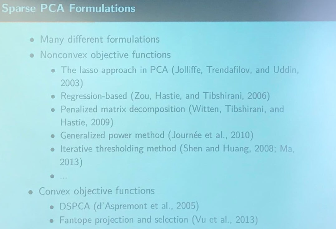
Sparse PCA Formulations
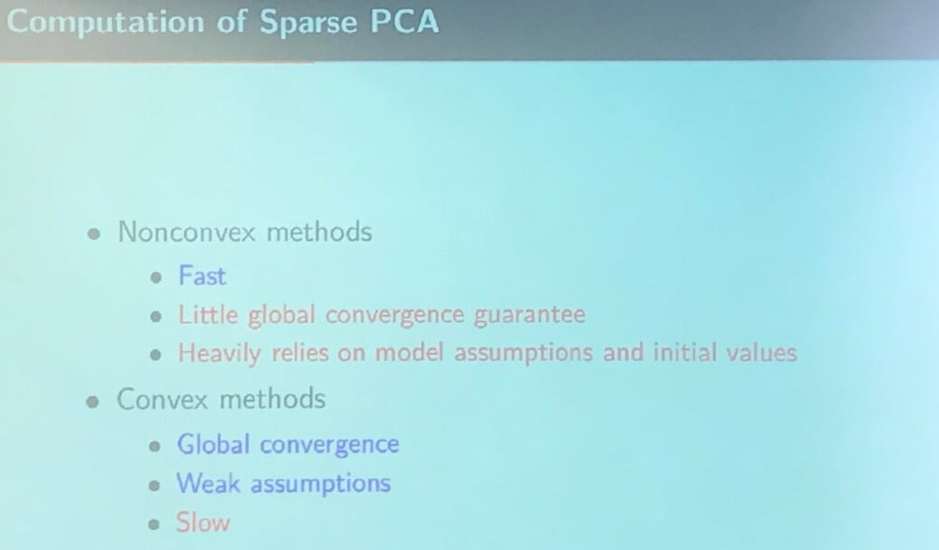
Computation of Sparse PCA
Model Setting
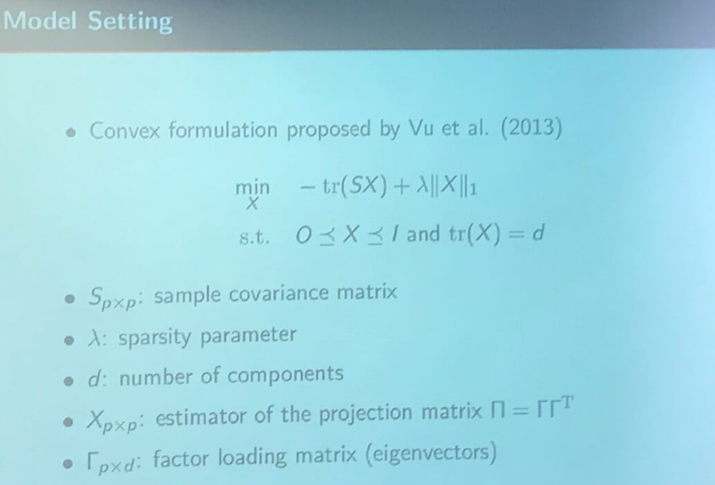
According to the original paper, the norm should be corrected to $\Vert X\Vert_{1,1}$, where \(\Vert A\Vert_{p, q} = \left\{\sum_{j=1}^n(\sum_{i=1}^m\vert a_{ij}\vert^p)^{q/p}\right\}^{1/q}\) denote the $L_{p,q}$ norm for an $m\times n$ matrix $A$.
The model is called Fantope projection and selection (FPS), and is equivalent to DSPCA as mentioned in the slide “Sparse PCA Formulations”.
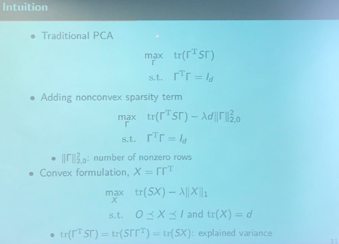
Intuition
Existing Computation Method
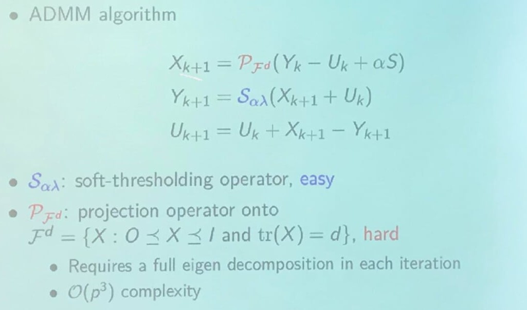
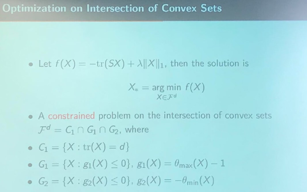
Optimization on Intersection of Convex Sets
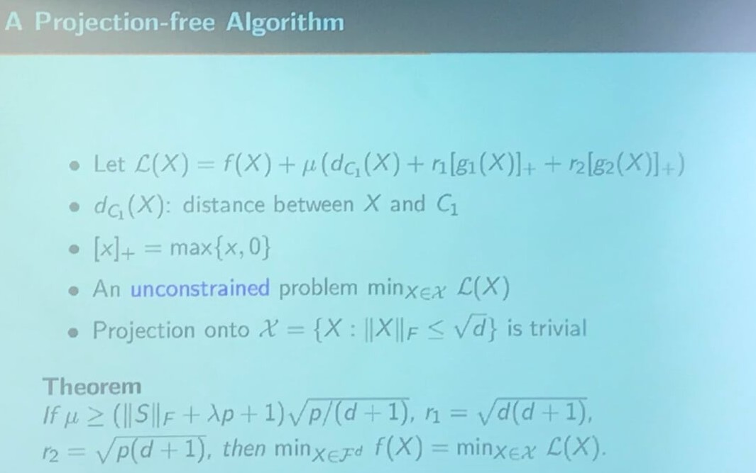
A Projection-free Algorithm
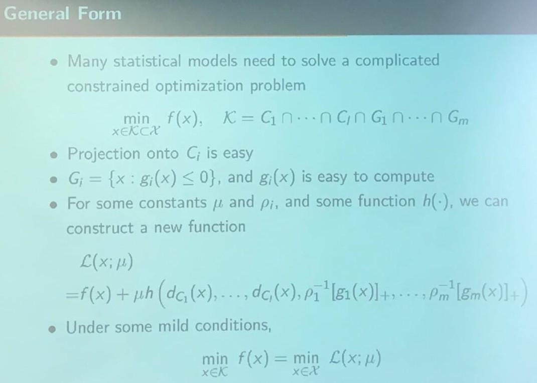
General Form
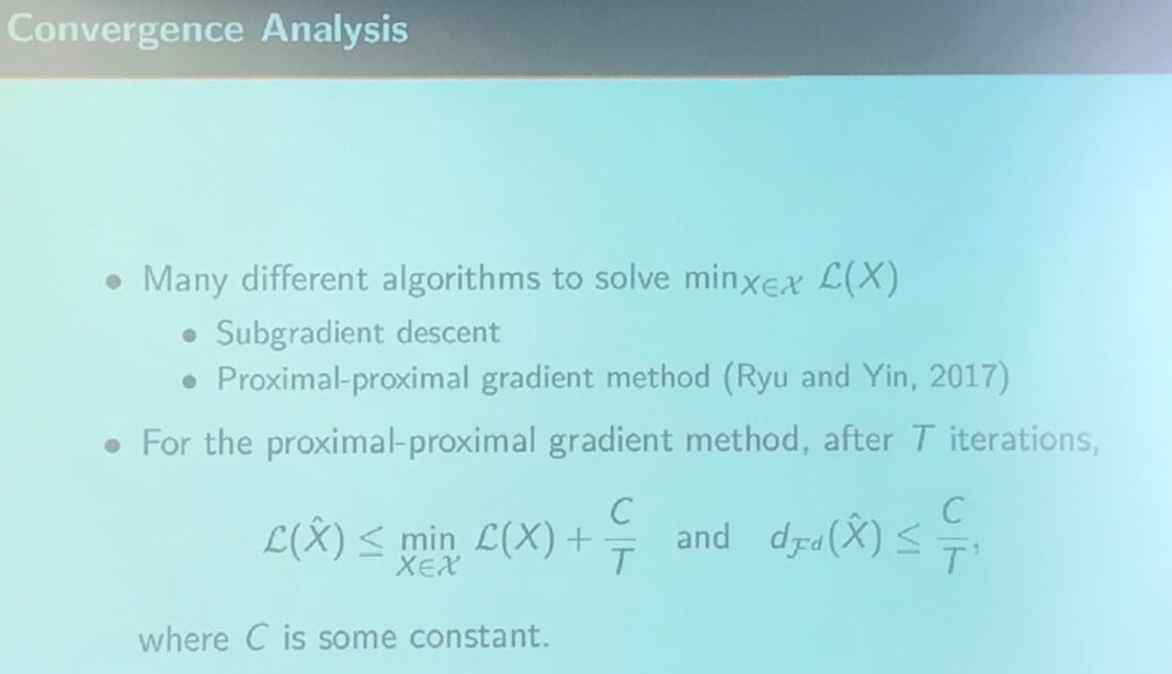
Convergence Analysis
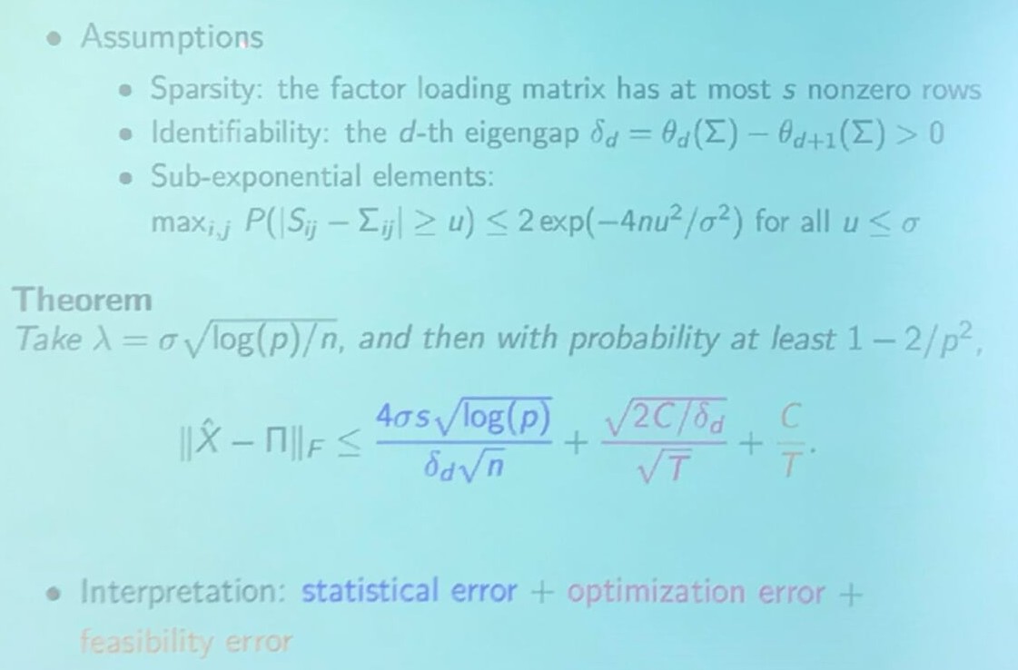
Statistical Property
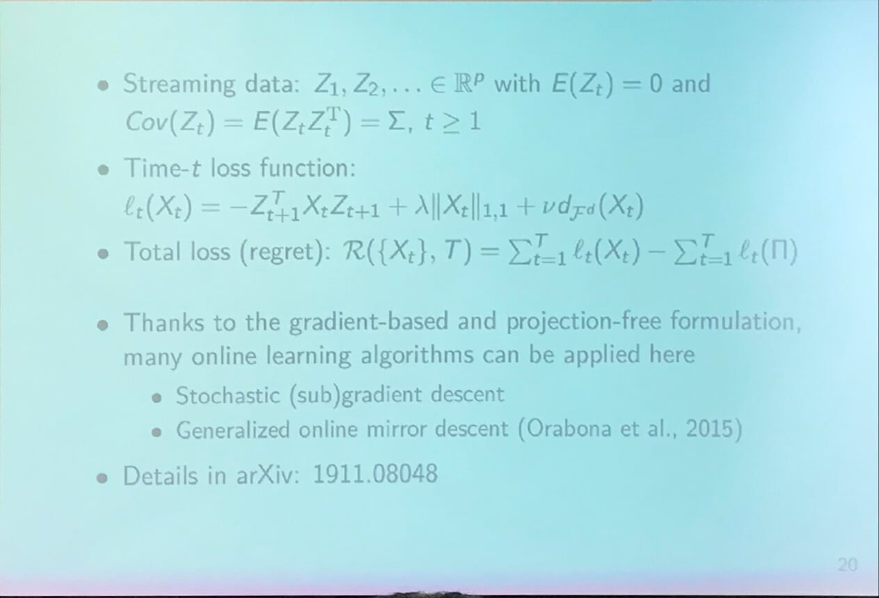
Extensions - Online Learning
More details refer to Gradient-based Sparse Principal Component Analysis with Extensions to Online Learning.
Computational Efficiency
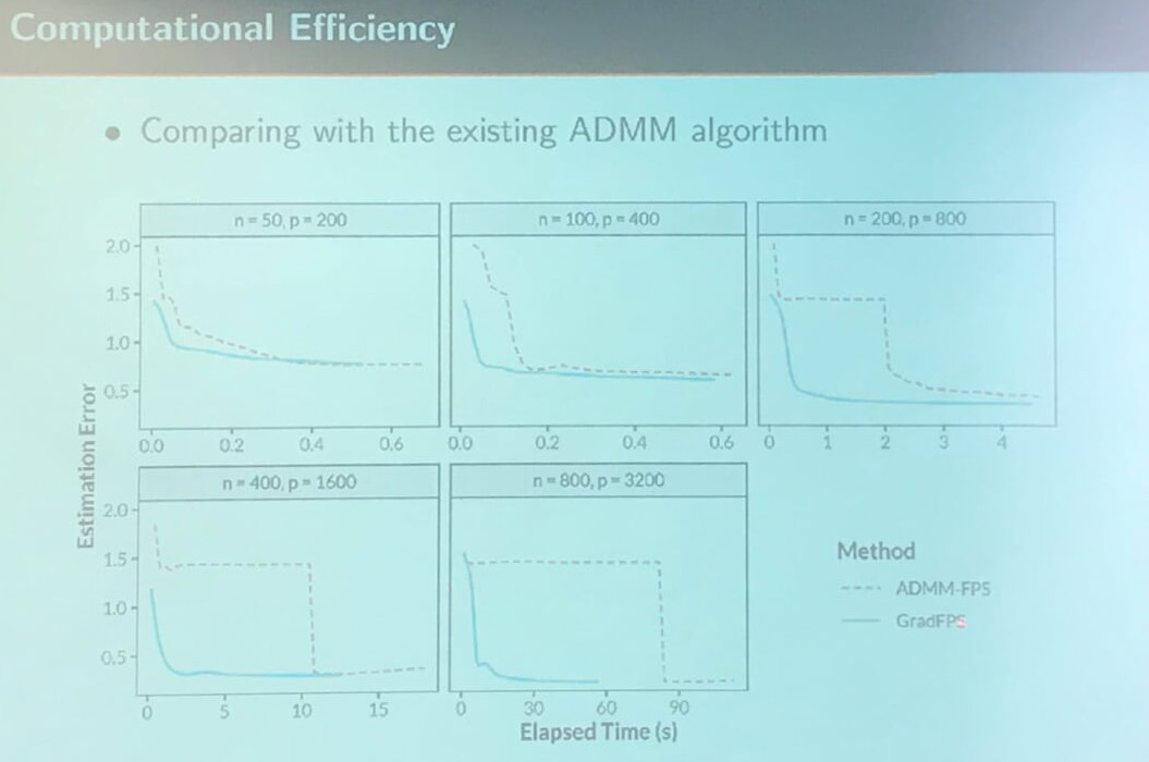
Here, I am wondering why ADMM-FPS would suddenly decrease the error, while the proposed method is more steadily.
Summary