Quantitative Genetics
Posted on (Update: )
This post is based on the Pao-Lu Hsu Award Lecture given by Prof. Hongyu Zhao at the 11th ICSA International Conference on Dec. 21th, 2019.
A Simple Model for Quantitative Traits
Connect phenotypes with genotypes (genetic factors)
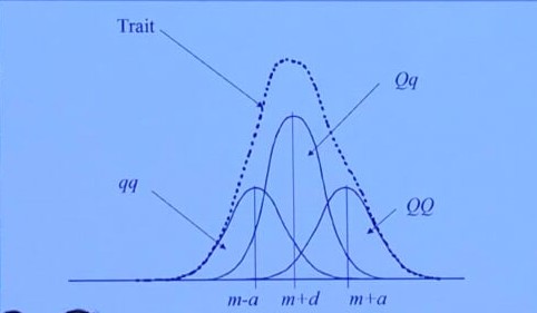
Consider a marker with two alleles (forms) $Q$ and $q$, with allele frequencies $f$ and $1-f$.
\[Y=G+E+e\]| Genotype | Value | Frequency |
|---|---|---|
| $QQ$ | $a$ | $f^2$ |
| $Qq$ | $d=0$ | $2f(1-f)$ |
| $qq$ | $-a$ | $(1-f)^2$ |
Partition of Genetic Variance
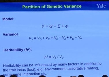
Heritability is a statistic used in the fields of breeding and genetics that estimates the degree of variation in a phenotypic trait in a population that is due to genetic variation between individuals in that population. Specifically, there are two detailed definitions:
- “narrow sense heritability” $h^2$: the proportion of trait variance that is due to additive genetic factors
- “broad sense heritability” $H^2$: the proportion of trait variance that is due to all genetic factors including dominance and gene-gene interactions.
Covariance between Relatives
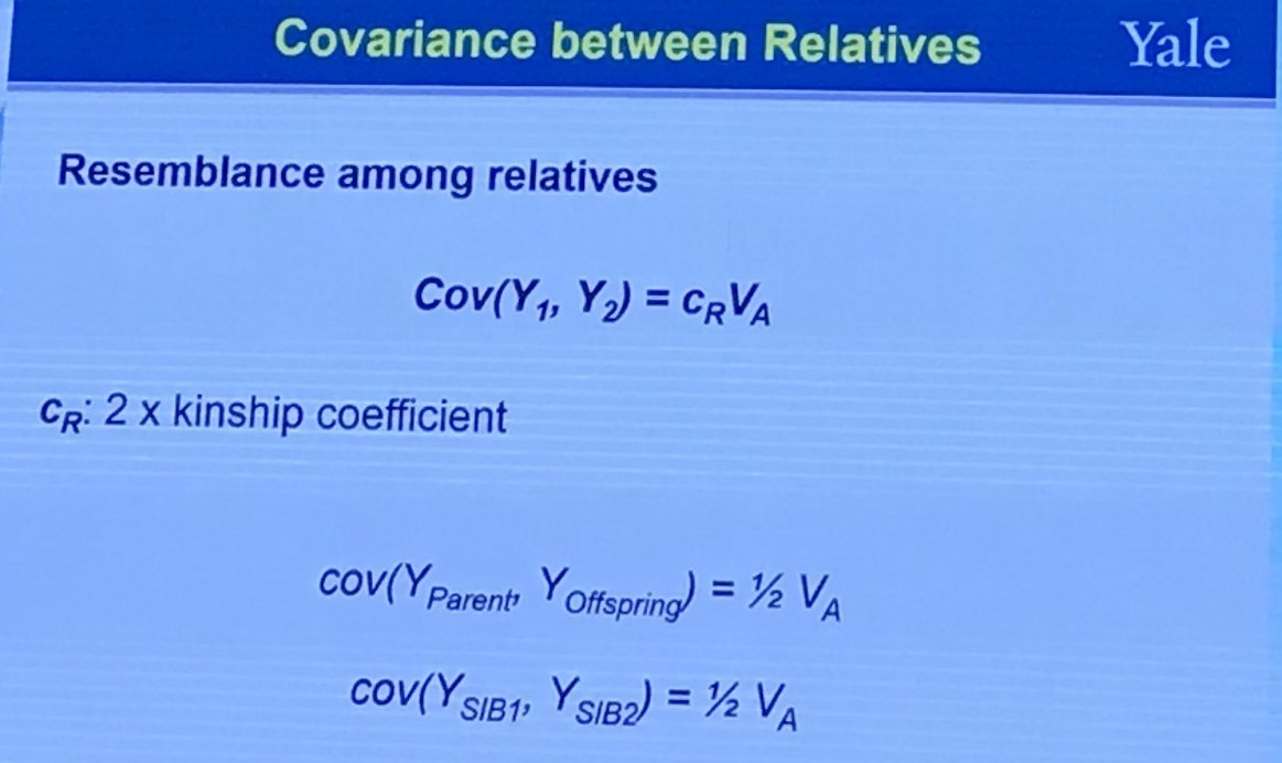
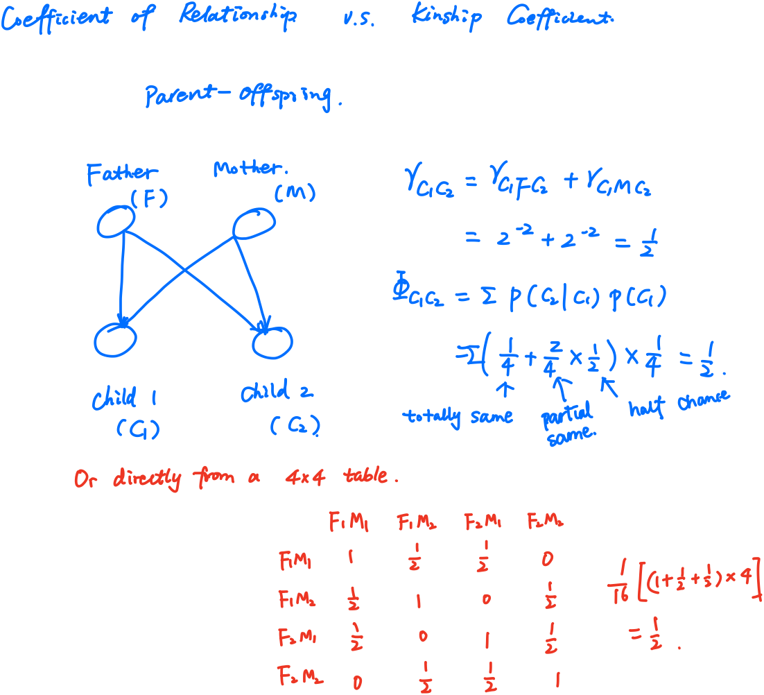
The coefficient of relationship $r$ between two individuals $B$ and $C$ is obtained by a summation of coefficients calculated for every line by which they are connected to their common ancestors (no more than one common ancestor). A path coefficient between an ancestor $A$ and an offspring $O$ separated by $n$ generations is given by
\[p_{AO} = 2^{-n}\left(\frac{1+f_A}{1+f_O}\right)^{1/2}\,,\]where $f_A$ and $f_O$ are the coefficients of inbreeding for $A$ and $O$, respectively. Hence,
\[r_{BC} = \sum p_{AB}\cdot p_{AC}\,.\]If $f=0$, it can be simplified to
\(r_{BC} = \sum_p2^{-L(p)}\,,\) where $p$ enumerates all paths connecting $B$ and $C$ with unique common ancestors.
The kinship coefficient is defined as the probability that a pair of randomly sampled homologous alleles are identical by descent (IBD). Simply, it is the probability that an allele selected randomly from an individual, $i$, and an allele selected at the same autosomal locus from another individual, $j$, are identical and from the same ancestor.
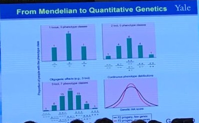
From Mendelian to Quantitative Genetics
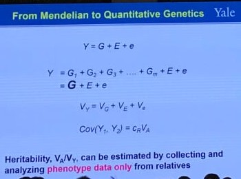
This corresponds to the way of plotting (or regressing) children’s traits against the average of their parents, i.e., the regression of offspring on the midparent. The reason is that, in the comparison of relatives,
\[h^2 = \frac br\,,\]where $b$ is the coefficient of regression and $r$ is the coefficient of relatedness (see the following definition). For parent-offspring regression, $r=1/2$, but for midparent-offspring regression, $r=1$, and hence the slope of the midparent-offspring regression is an estimate of heritability.
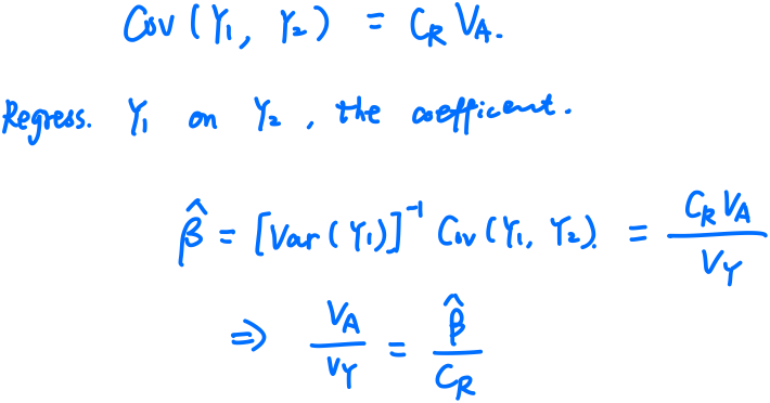
Here is a clearly-stated post which explains why the slope, not the variance explained, allows estimation of heritability
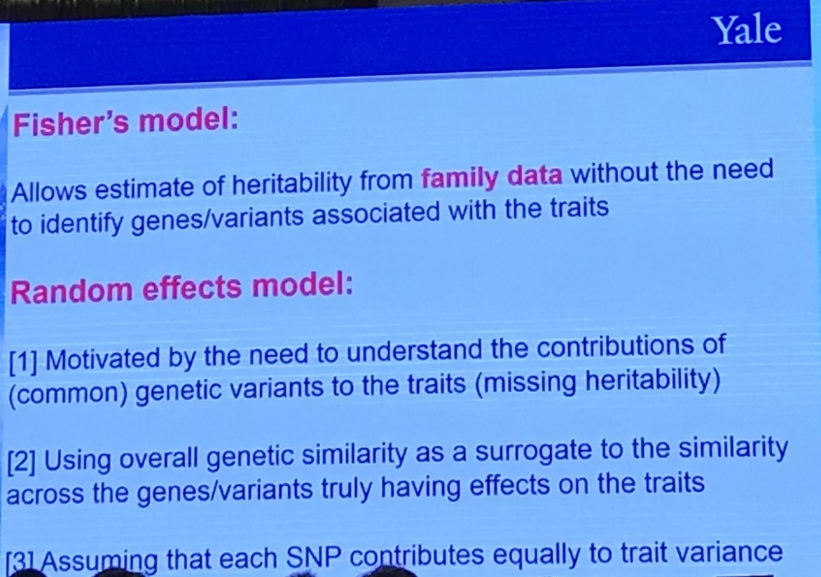
Note that we can estimate heritability without knowing which genes contribute to traits of interest if we assume the genetics model is correct (Fisher’s model).
However, it is reported that the problem with the (mid)parent-offspring regression is that parent and child share a lot else besides half their genome. One approach to calculating heritability which largely avoids the confounding of genotype with shared environment is to compare the phenotypic concordance of monozygotic (MZ, 同卵) twins versus dizygotic (DZ, 异卵) twins. Both types of twins are expected to share virtually all environment factors, and hence comparing MZ to DZ twins lets you isolate the contribution of that marginal half shared genome to phenotypic concordance. The associated statistic is called Falconer’s formula,
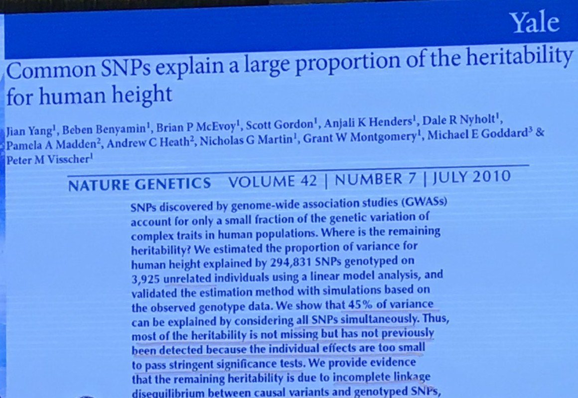
\[\text{heritability} = 2(r_{MZ}-r_{DZ})\,.\]Genome Wide Association Studies
GWAS General strategy:
- Thousands up to hundreds of thousands of subjects
- Genome wide markers, up to several millions
- Correlate SNP with phenotypes to identify markers significantly associated with the phenotypes
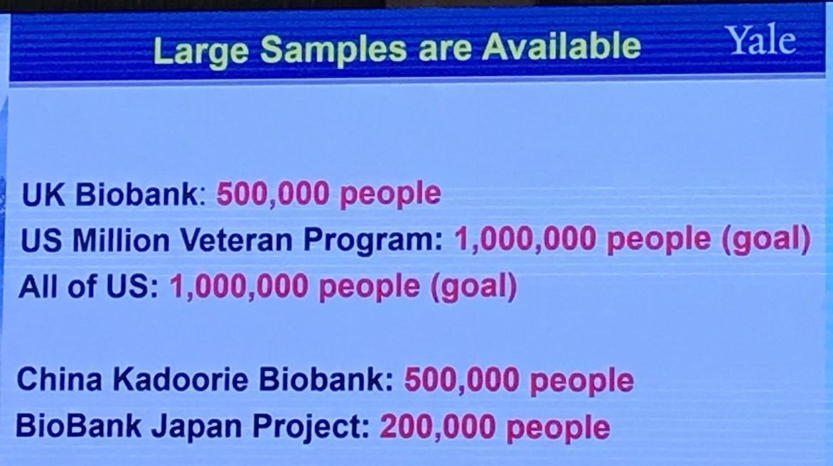
Large Samples are Available
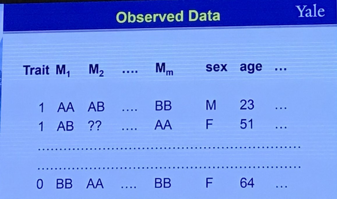
Observed data
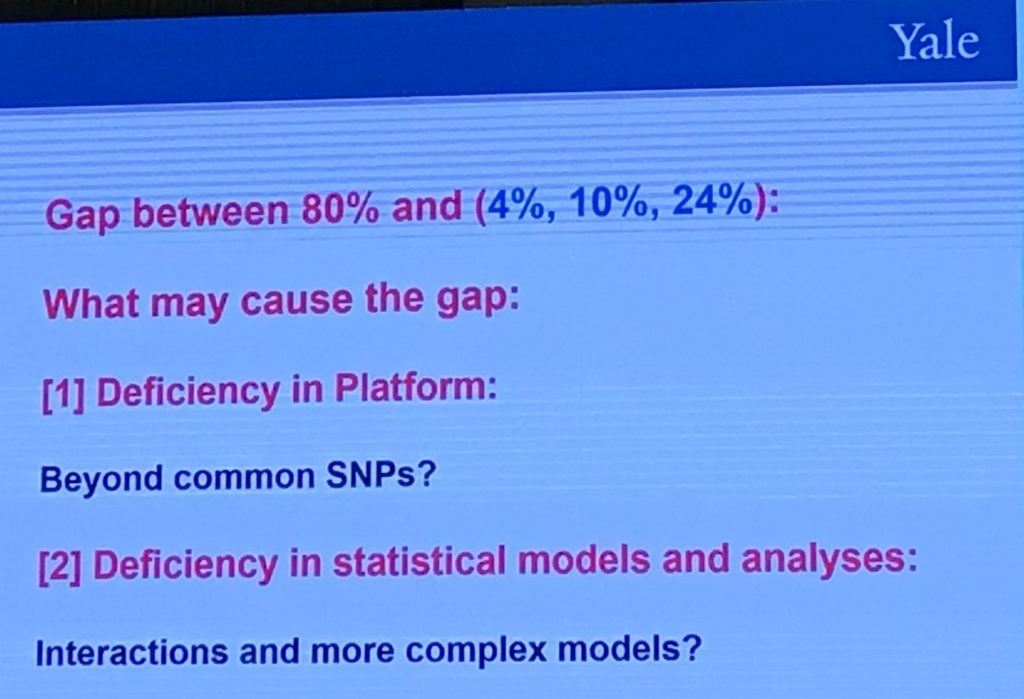
One Question to Ask
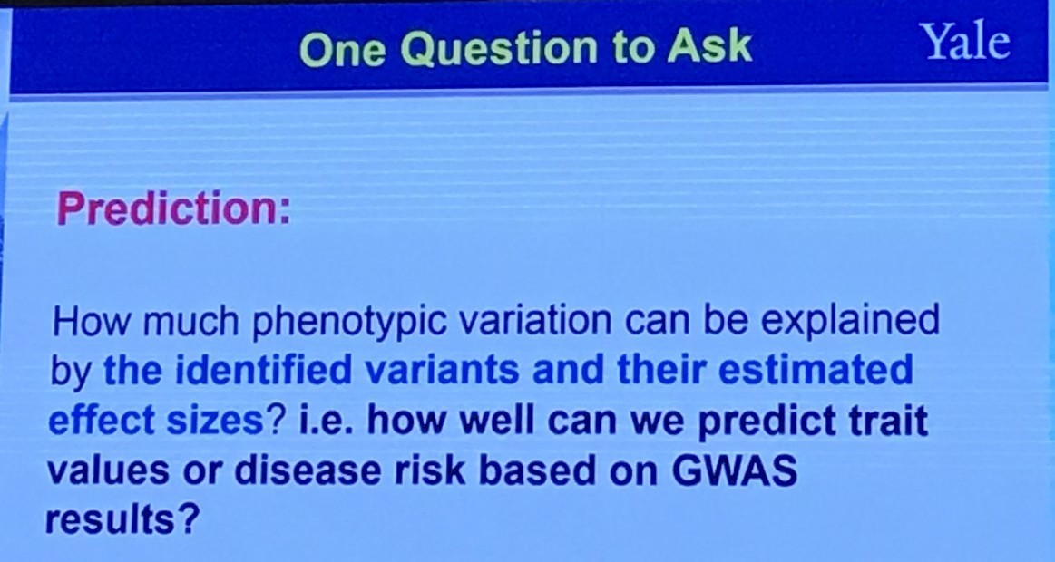
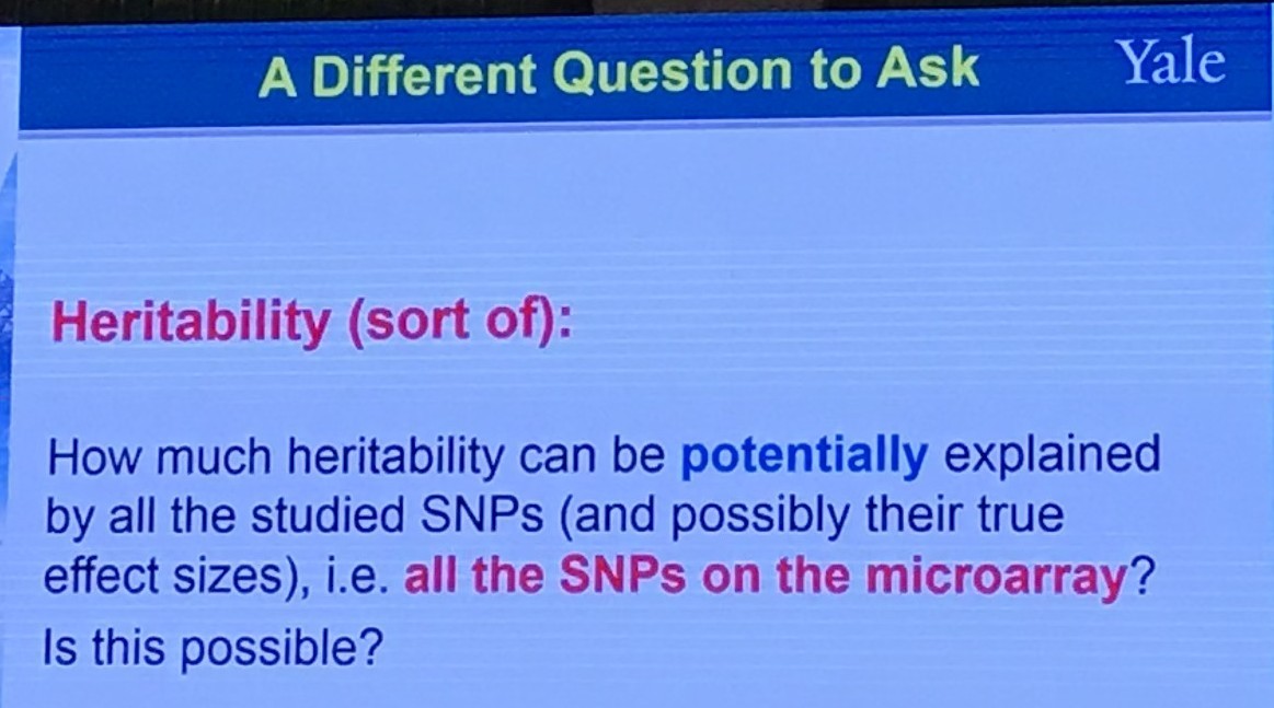
A Different Question to Ask
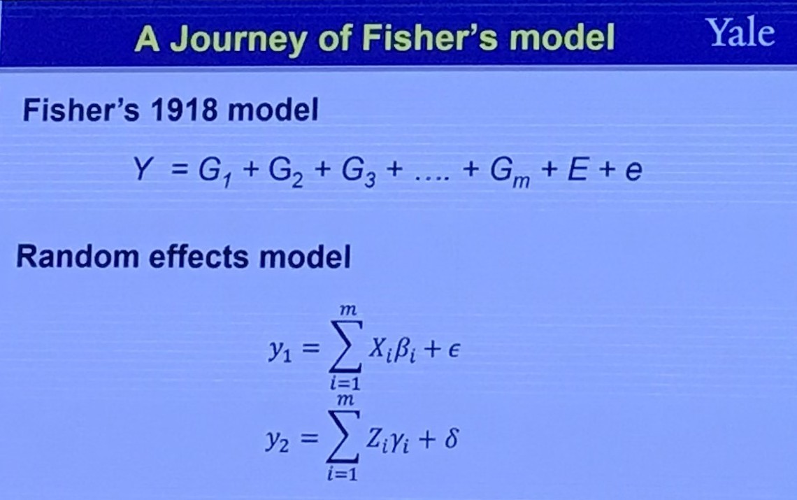
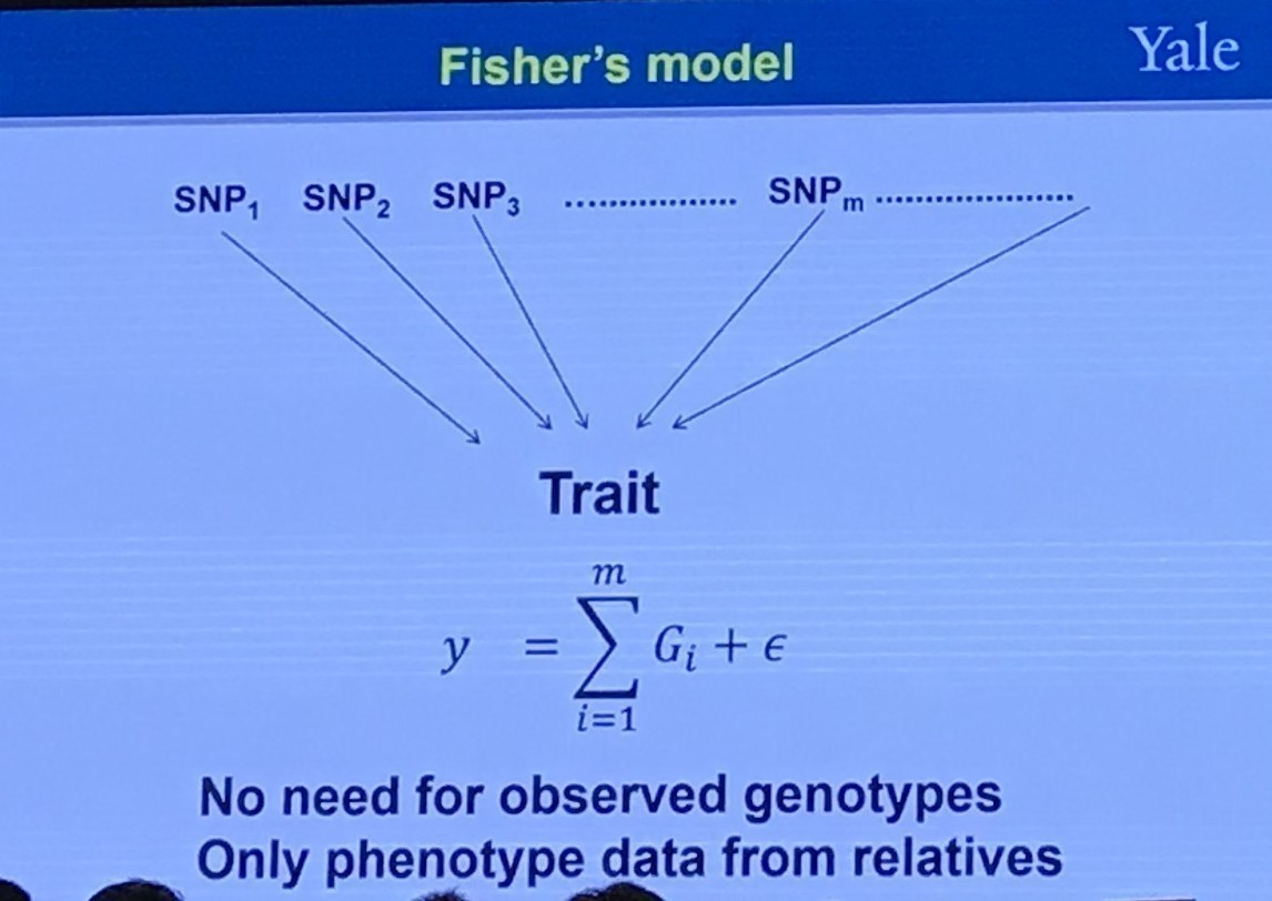
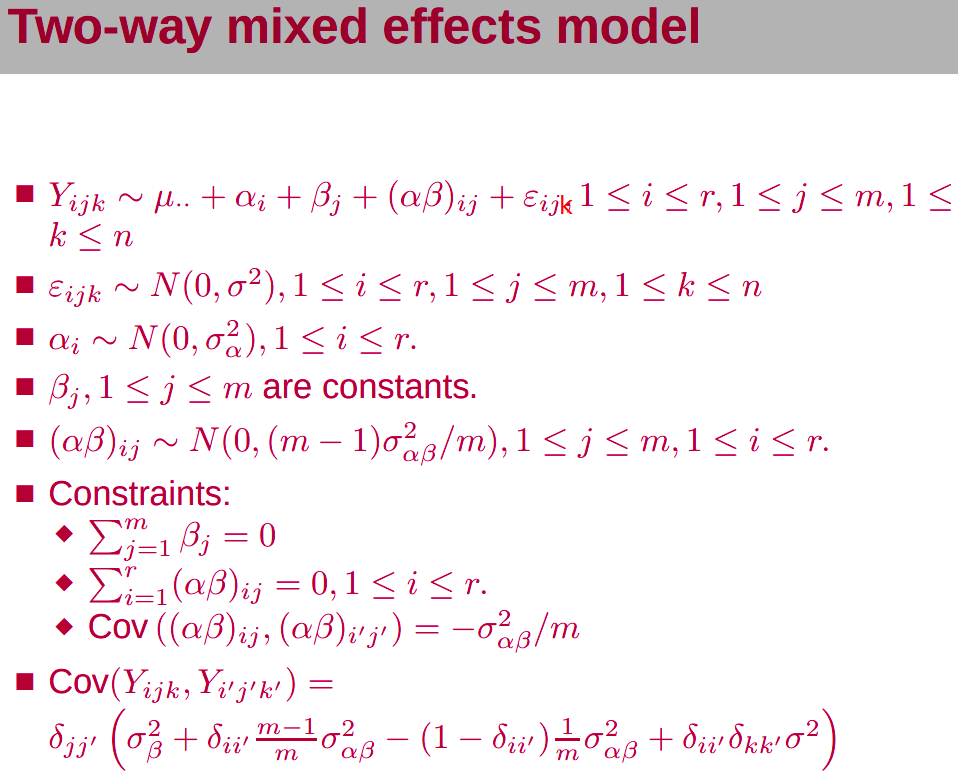
Fisher’s Model
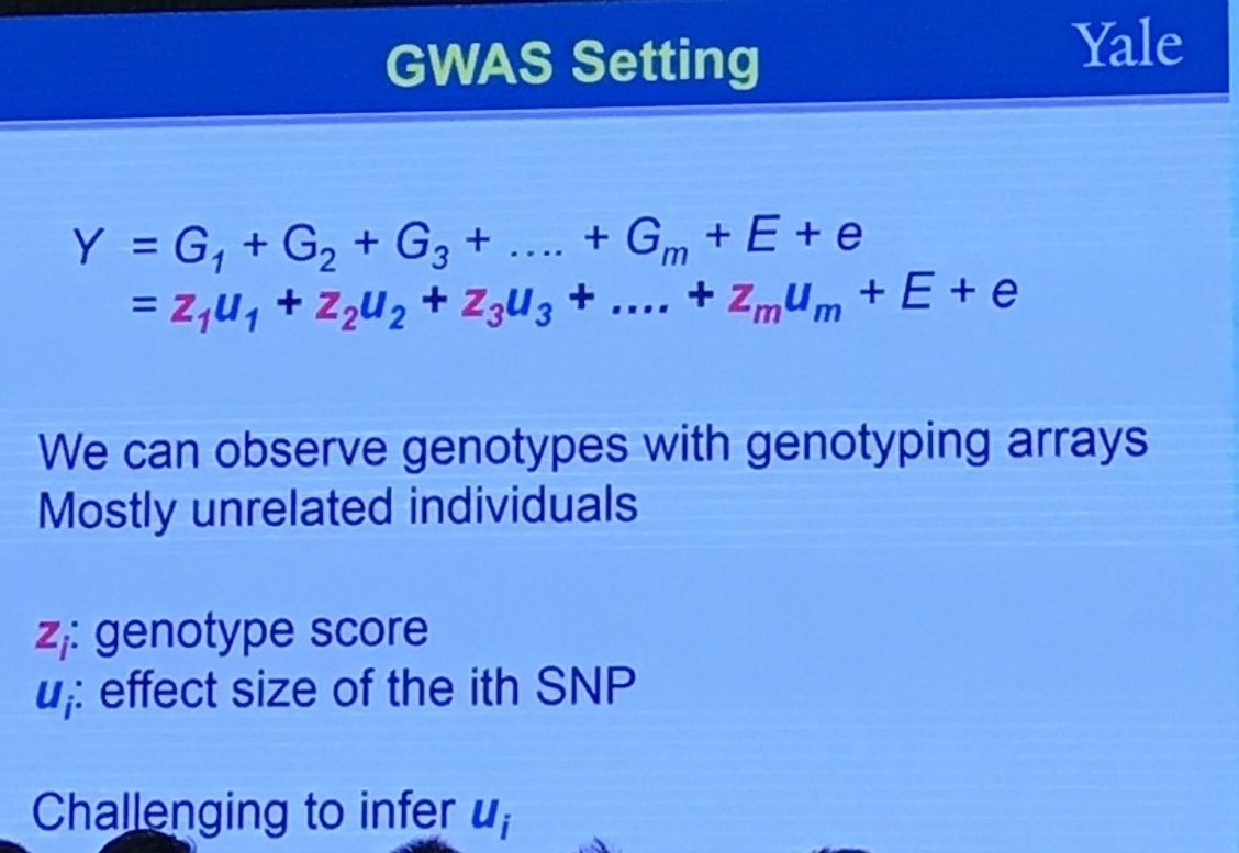
GWAS Setting
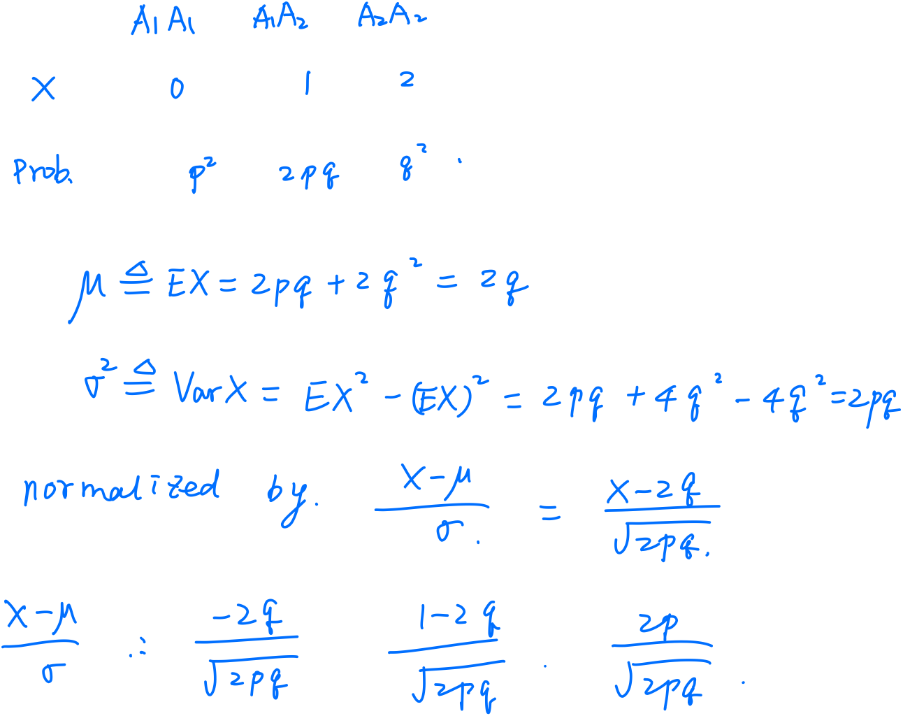
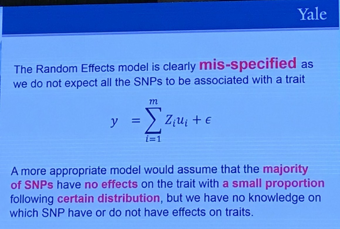
Random Effects Model
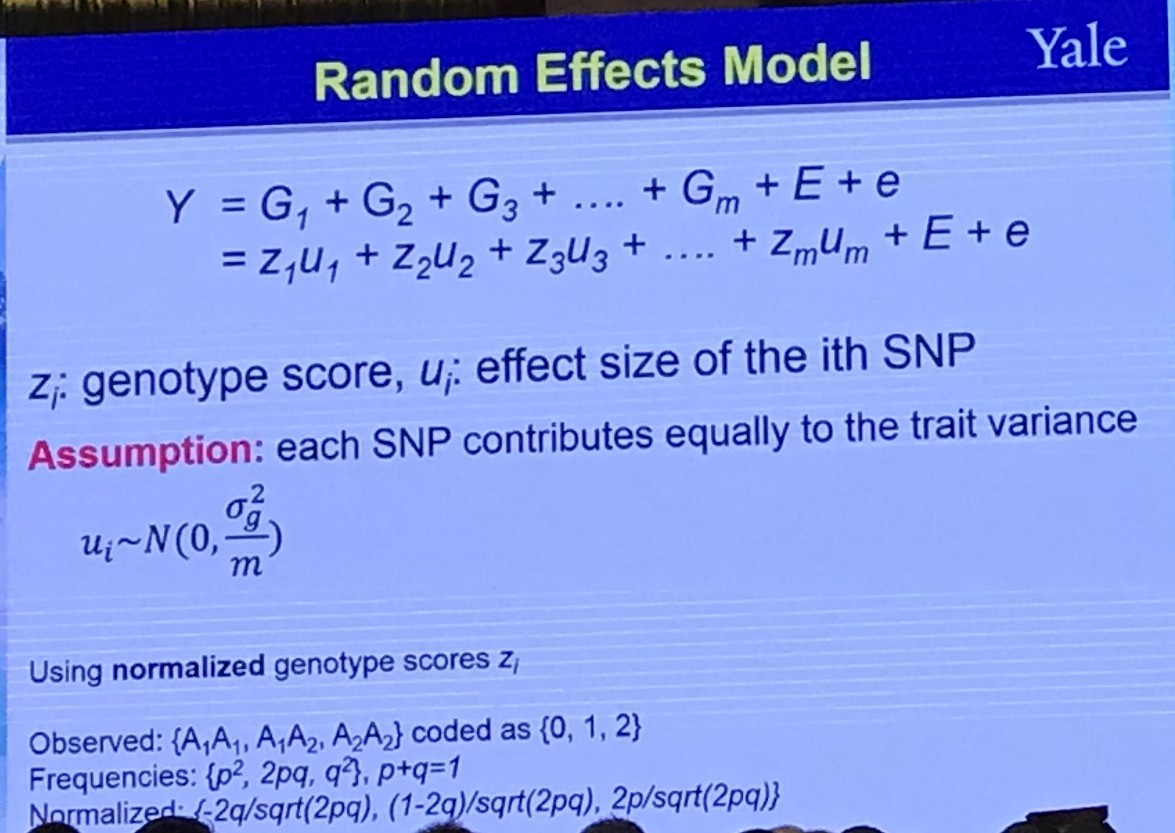
A “group” effect is random if we can think of the levels we observe in that group to be samples from a larger population.
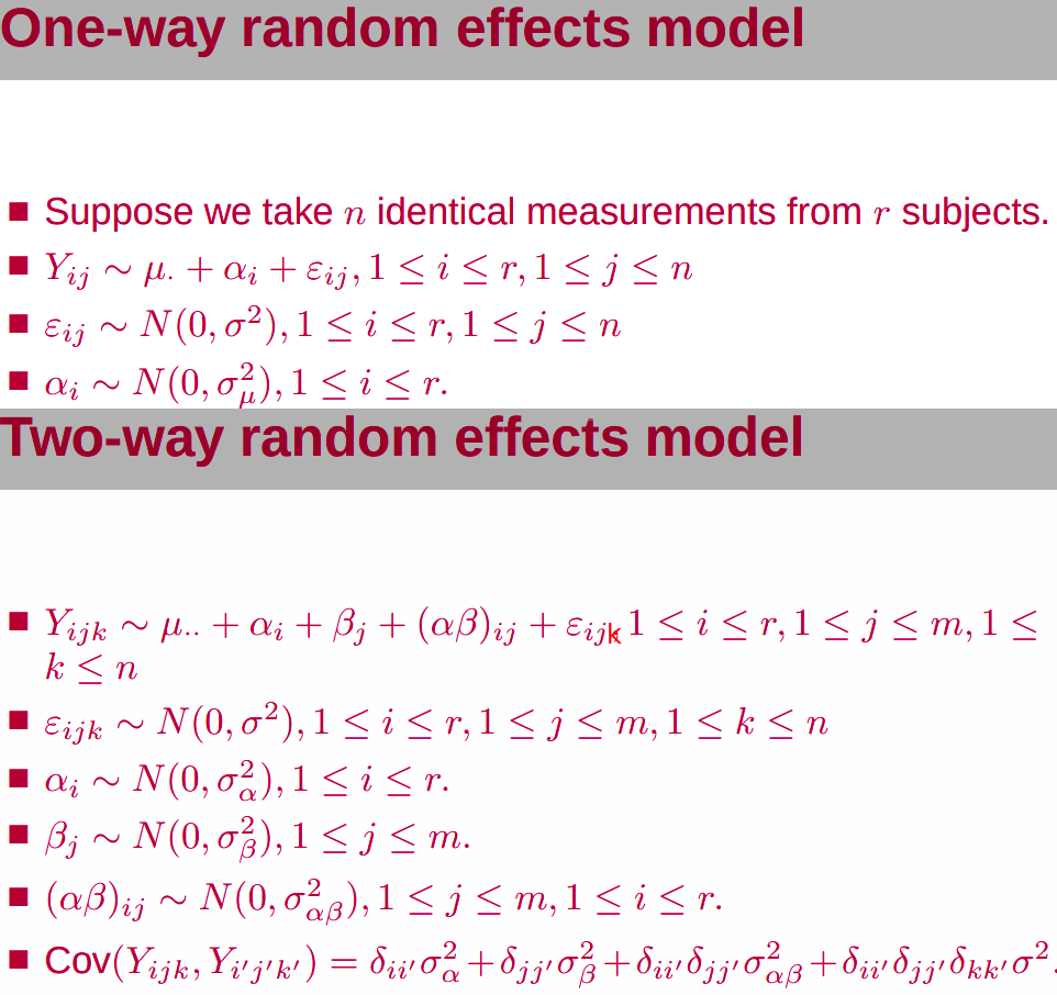
In some studies, some factors can be thought as fixed, others random.
adopted from Statistics 203: Introduction to Regression and Analysis of Variance – Fixed vs. Random Effects
Back to the slide, I am a little confused, where there is only one index, $i$, represents subject or repeated measurement? If for different subjects, what is the repeated measurement since there should be some samples for a particular subject. If for repeated measurement, does it mean that only 1 subject, and treat different individual as a “repeated” measurement for each gene (SNP)?
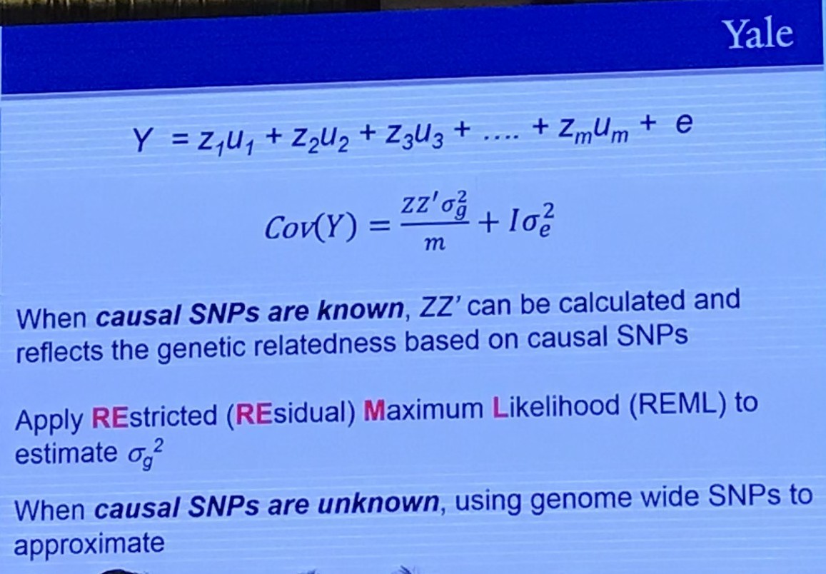
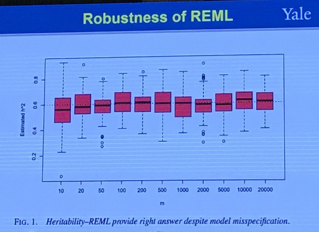
The Restricted (or Residual, or Reduced) maximum likelihood (REML) approach is a particular form of maximum likelihood estimation that does not base estimates on a maximum likelihood fit of all the information, but instead uses a likelihood function calculated from a transformed set of data, so that nuisance parameters have no effect.
Is there some connection with conditional MLE, c.f. A8 of STAT5010?
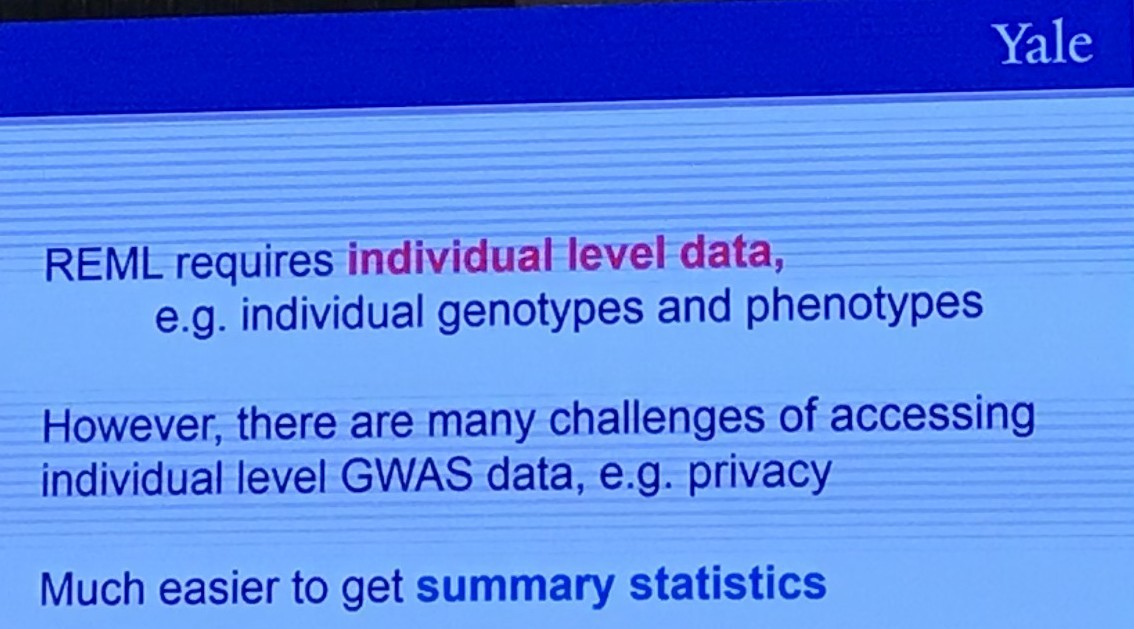
Individual Level vs Privacy
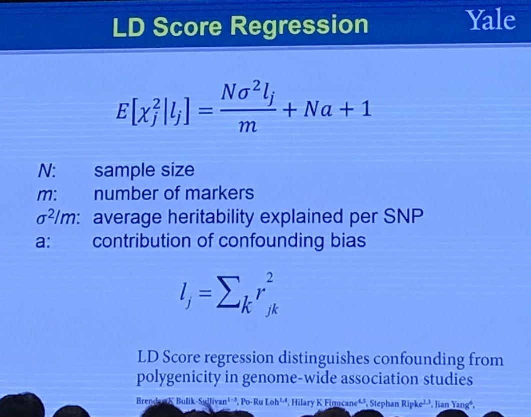
It is claimed that the LD score regression can quantify the contribution of each polygenicity (many small genetic effects) signal and bias by examining the relationship between test statistics and linkage disequilibrium (LD).
The level of linkage disequilibrium between allele $A$ and a different locus allele $B$ can be quantified by the coefficient of linkage disequilibrium
\[D_{AB} = p_{AB} - p_Ap_B\,.\]
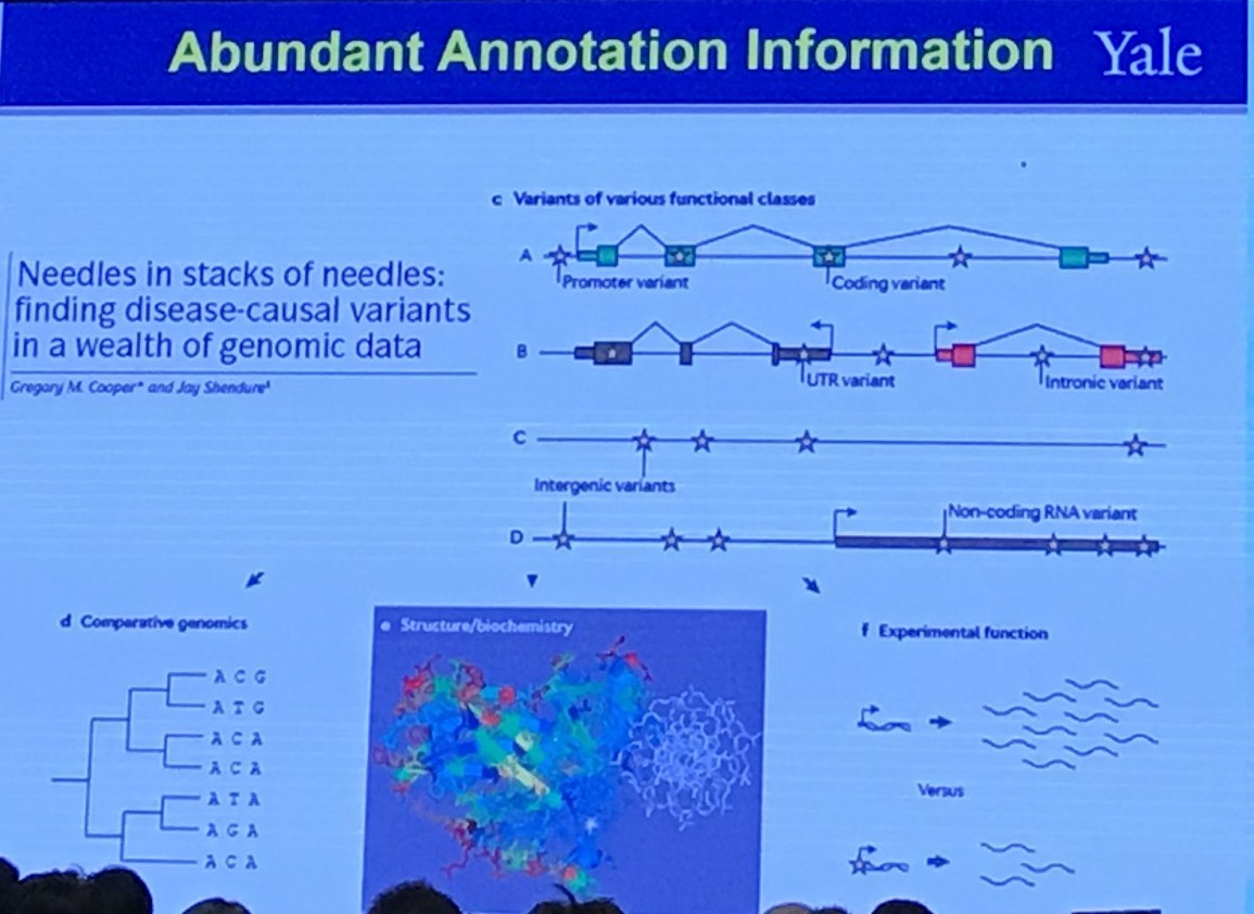
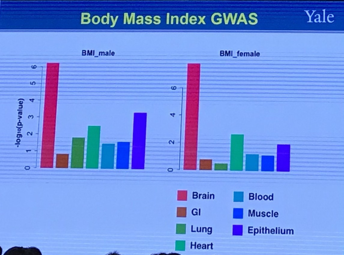
Abundant Annotation Information
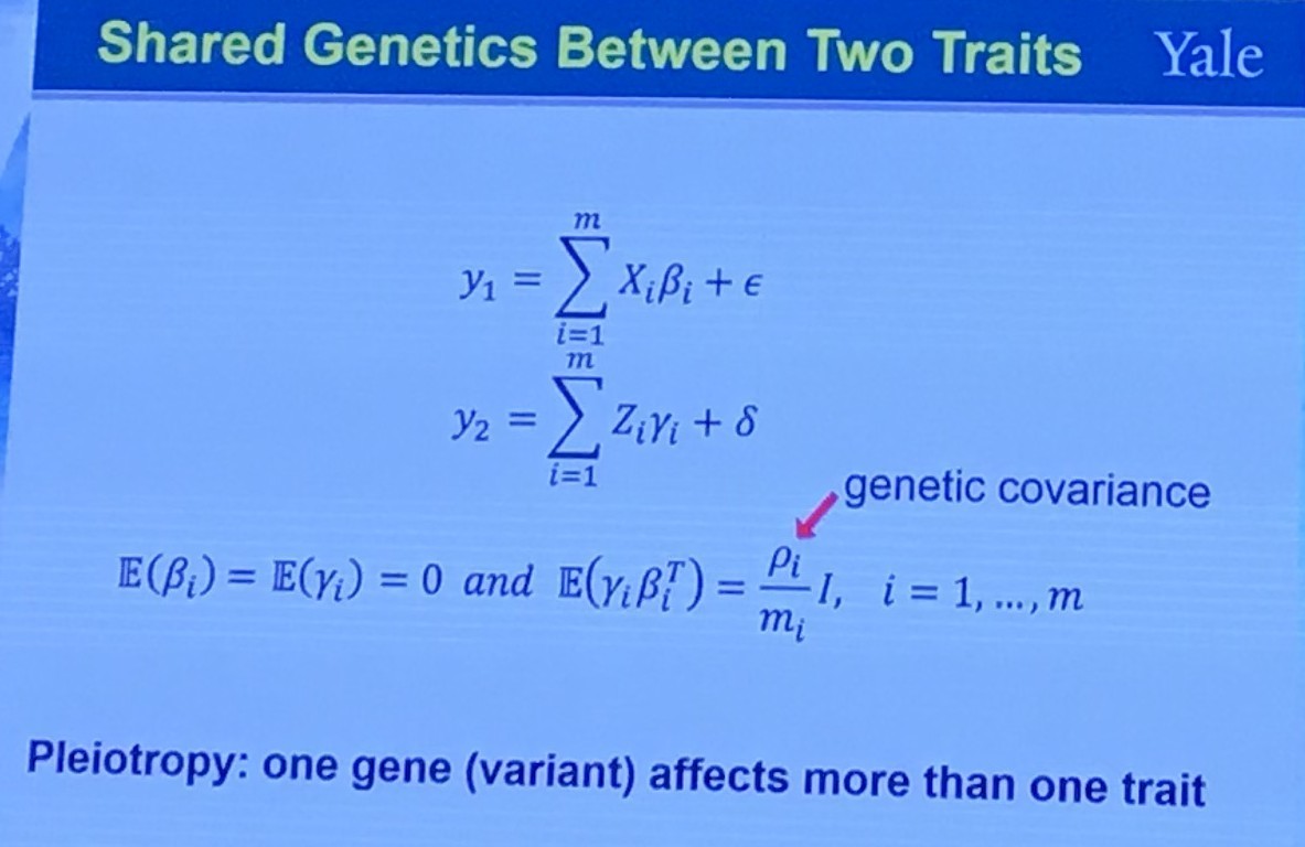
Shared Genetics Between Two Traits
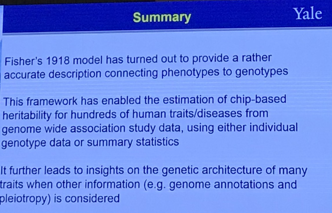
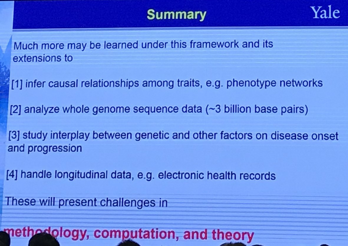
Summary