Conditional Quantile Regression Forests

Posted on Dec 12, 2019

Tags: Random Forests, Quantile Regression

This note is based on the slides of the seminar, Dr. ZHU, Huichen. Conditional Quantile Random Forest.

Motivation

REactions to Acute Care and Hospitalization (REACH) study

• patients who suffer from acute coronary syndrome (ACS, 急性冠心症) are at high risk for many adverse outcomes, including recurrent cardiac (心脏的；心脏病的；心脏病患者) events, re-hospitalizations, major mental disorders, and mortality. There is an urgent need for post-discharge (出院后) chronic (长期的，慢性的) care for ACS patients.
• developing accurate predictive models for those adverse events are the first step in response to such need.
• The Columbia University Medical Center has established an on-going cohort since 2013, called the REactions to Acute Care and Hospitalization (REACH)
  • Includes rich and comprehensive electronic medical records (EMRs) of 1744 ACS patients
  • Provides a unique and ideal platform to develop high-dimensional statistical predictive analysis for ACS patients.

Scientific/Clinical Objectives

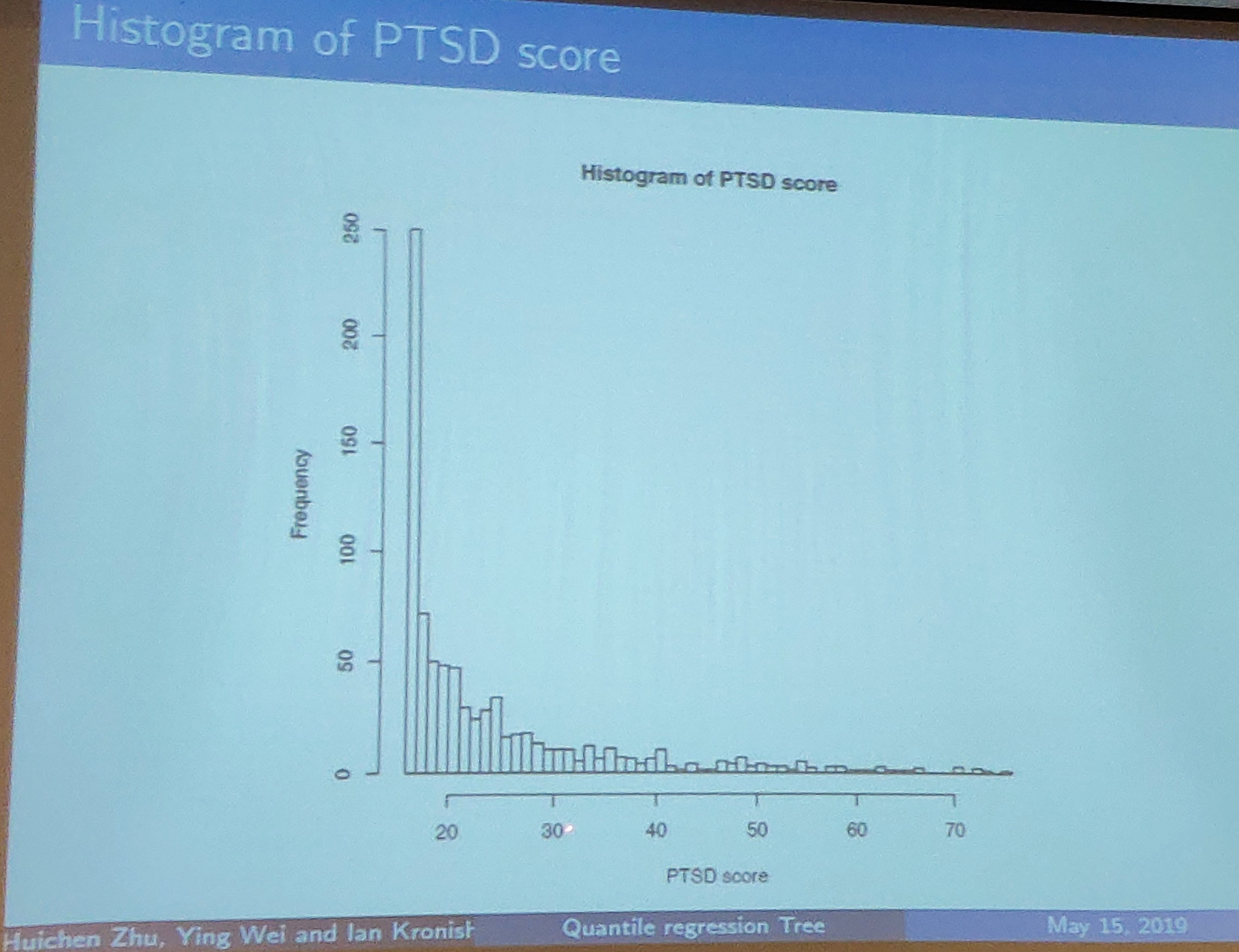
• one of the adverse event is post-traumatic stress disorder (PTSD), which leads to a much higher risk of recurrent cardiovascular (心血管的) events and mortality.
• about 20% of the patients in REACH cohort achieved a higher score based on a PTSD checklist within one month after emergency room (ER) discharge
• goal: to develop a statistical approach to enhance the prediction of PTSD at the time of discharge

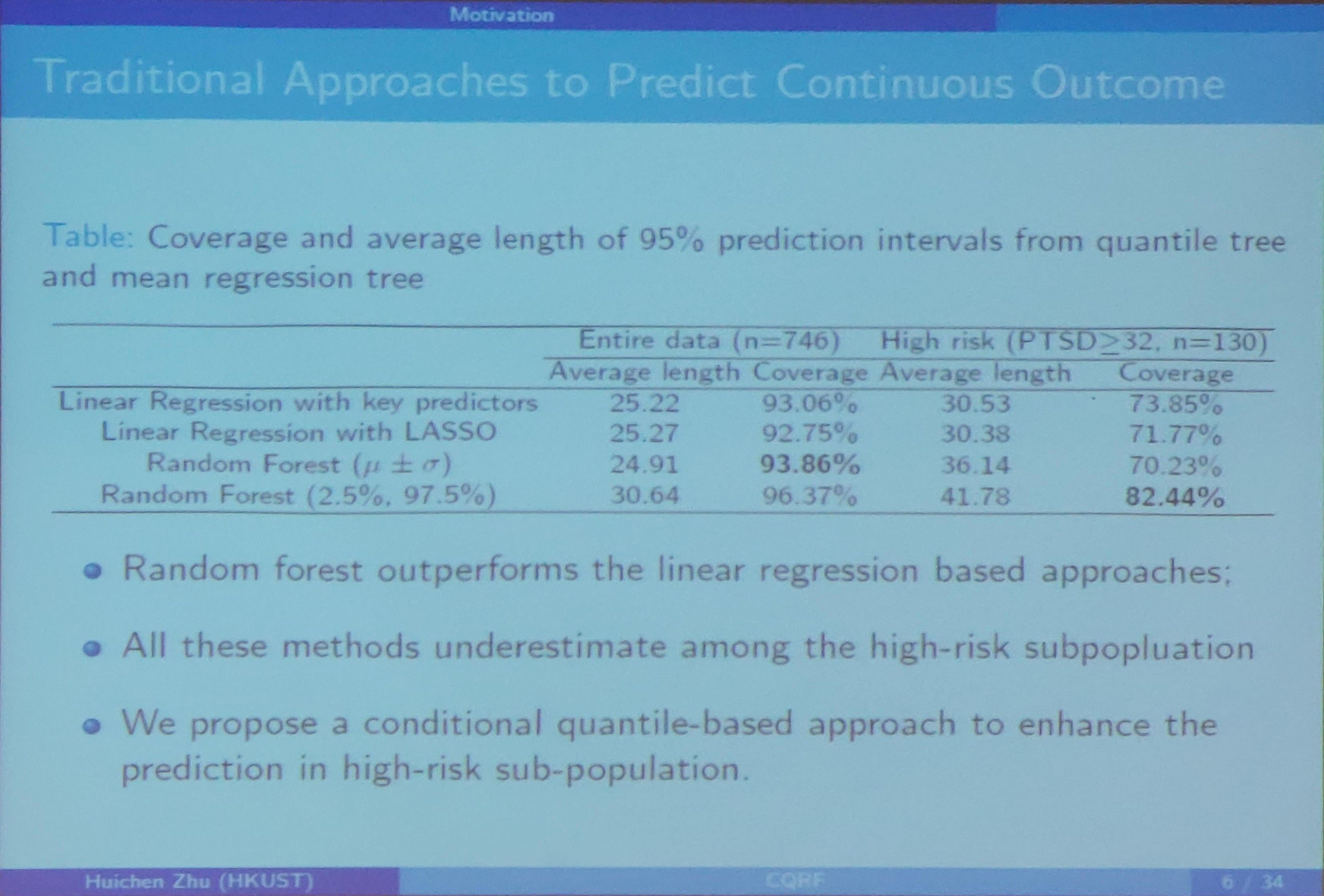
Traditional Approaches to Predict Continuous Outcome

1. Linear Regression
   • with a set of pre-specified key predictors
   • with variable screening and selection to include a large number of potential predictors
     • LASSO
     • SCAD
     • elastic net
2. Machine learning approach
   • random forest
   • support vector machine
   • linear discriminant analysis
   • k-means clustering

Quantile Regression

• Conditional quantile: $Q_\tau(Y\mid X)=\inf\{y:\Pr(Y\le y\mid X)\ge \alpha\}$
• Quantile regression (Koenker & Bassett Jr, 1978) is an extension of traditional linear regression
• Quantile regression allows us to study the impact of predictors on different quantiles of response distribution, and thus provides a complete picture of relationship between $Y$ and $X$.

Combine the Domain Knowledge

• Theoretical mental health for ACS survivor indicates that PTSD due to a medical event is often driven by the fear of death and recurrence
• The impact of the fear also depends on individuals
• REACH study have assessed the fear level using multiple measures during emergency room (ER) visits
• Adopting such domain knowledge into the data-driven machine learning approach is potentially another direction to improve the prediction

(??Is that fair for the previous compared methods do not combine such domain knowledge)

Existing Works

Only a few previous work involving quantile related splitting criterion or prediction in regression tree or random forest.

• Chaudhuri and Loh (2002) and Bhat et al. (2015) proposed to partition the sample using conditional quantile loss functions at a fixed quantile level
• Meinshausen (2006) proposed to use empirical functions for predictions, but individual tree is still based on CART

Proposed Methods

A Non-parametric Interactive Quantile Model for PTSD prediction

Assume a non-parametric interactive quantile model

\[Q_{y_i}(\tau, x_i, z_i) = \beta_0(\tau, x_i) + z_i^T\beta_1(\tau, x_i)\,,\]

where

• $y_i$: individual post-ACS PTSD scores
• $z_i$: key predictors (level of fear during ER visit, PTSD score at baseline)
• $x_i$: a $p$-dimensional patient profile from EMR
• $\tau\in (0,1)$: the quantile level

Splitting Criterion

• For any recursive partition approach, a splitting criterion is the most crucial part.
• Classical regression tree/forest choose the optimal split that leads to the greatest reduction in Residual Sum of Squares (RSS).
• It partitions the sample into subsets with distinctive means.

Conditional Quantile-based Splitting Criterion I

Step 1

First determine a $K$ that $\tau_k = k/(K+1),k=1,2,\ldots,K$. Build a quantile regression model for each $\tau_k$ at node $N$ as

\[Q_y(\tau_k,z,x\in N) = z^T\beta_N(\tau_k, 0)\,,\]

where $\beta_N(\tau_k, 0)$ is the quantile coefficient at quantile level $\tau_k$. (?? confused about the notation, why take 0 as the second argument, got the idea in the following context). Estimate each $\beta_N(\tau_k, 0)$ by

\[\hat\beta_N(\tau_k, 0) = \argmin_\beta L_N(0, \tau_k, \beta) = \argmin_\beta \frac{1}{\vert N\vert}\sum_i\rho_{\tau_k}(y_i-z_i^T\beta)I(x_i\in N)\,.\]

Step 2

Re-model the data in $N$ following the split $s$ as

\[Q_Y(\tau, z_i, s) = z_i^T\beta_1(\tau, s) + \delta_i(s)z_i^T\beta_2(\tau, s)\,,\]

where $\beta_N(\tau, s) = (\beta_1(\tau, s)^T, \beta_2(\tau, s)^T)^T$ represents the quantile coefficients following the partition $s$, and

\[\delta_i(s) = \begin{cases} 1 & \text{$x_i$ belongs to the resulting left child node $N_L^s$}\\ 0 & \text{o.w.} \end{cases}\]

Estimate each $\beta_N(\tau_k, s)$ by

\[\hat \beta_N(\tau_k, s) = \argmin_\beta L_N(s,\tau_k, \beta) = \argmin_{\beta_1,\beta_2} \frac{1}{\vert N\vert} \sum_i[\rho_{\tau_k}\left\{y_i - z_i^T\beta_1 - \delta_i(s)z_i^T\beta_2\right\}I\left\{x_i\in N\right\}]\,.\]

So, it seems that $\beta_1+\beta_2$ for the left child node, while $\beta_1$ for the right child node.

Step 3

Propose the first splitting criterion, extended from the concept of RSS, in the form,

\[\Delta_N(s) = \sum_{k=1}^K\omega(\tau_k) \left\{ \frac{\hat L_N(0, \tau_k) - \hat L_N(s, \tau_k)}{\hat L_N(0, \tau_k)} \right\}\,,\]

where $\hat L_N(s,\tau_k) = L_N(s, \tau_k, \hat\beta(\tau_k, s))$. The term $\omega(\tau_k)$ is a predefined weight function and reflects the relative importance across quantile levels.

Step 4

Choose the optimal split by maximizing $\Delta_N(s)$, set

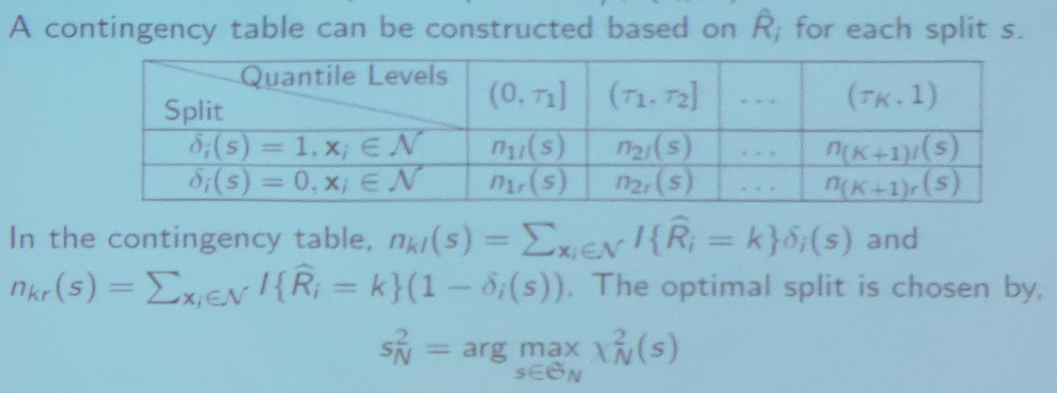
\[s_N^1 = \argmax_{s} \Delta_N(s)\,.\]

Splitting Criterion II

Let

\[\hat \beta_N(\tau_k, 0) = \argmin_\beta L_N(0, \tau_k, \beta)\,.\]

Denote that

\[\hat R_i = \sum_{k=1}^K I\left\{ y_i-z_i^T\hat \beta_N(\tau_k, 0) \le 0\right\}\,,\]

which ranges between 1 and $K$ and identifies the rank of $y_i$ with respect to the estimated conditional quantile process (?? due to $k$?) $z_i^T\hat\beta(\tau_k, 0)$.

A contingency table can be constructed based on $\hat R_i$ for each split $s$.

Comparing the Splitting Criteria

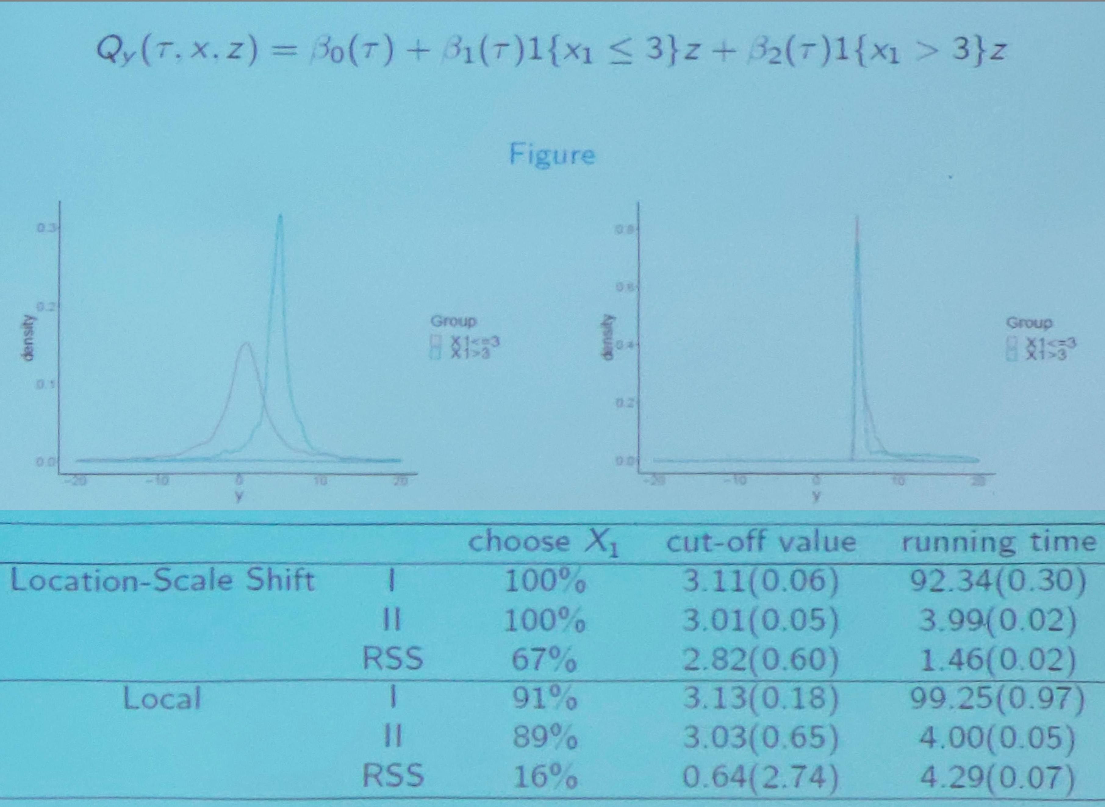
confused about the above two figures.

Algorithm for Conditional Quantile Random Forest

Let $(y_i, x_i, z_i), i=1,\ldots, n_t$ be a training data.

Step 1: Sub-sampling the training data

randomly draw a sub-sample ($m, m\le n_t$ out of $n_t$ samples without replacement) from the training data (not a bootstrap sample!？)

Step 2: Grow a tree

based on the sub-sample, at each split

1. randomly draw $p^*\le p$ out of $p$ predictors $x$ as the potential splitting variables ($p^*$ is pre-specified number)
2. select the optimal splitting variable using the rank score test statistics
3. select an optimal cut-off value of the splitting variable using the proposed criterion

Step 3: Assemble a random forest

The Applications of CQRF

Applications

• Prediction: a new patient with covariates profile $(x^*, z^*)$
  • first estimate the individualized conditional quantile effects $\beta(\tau, x^*)$ based on the constructed CQRF
  • construct the estimated conditional quantile process ${z^*}^T\hat\beta(\tau, x^*)$
  • based on the constructed conditional quantile function, we could obtain: prediction mean, prediction median, prediction interval and predicted risk assessment
• Feature selection: evaluate and rank the importance of the splitting variables
• Precision medicine: assessing individualized treatment effect

Estimating Algorithm of $\beta(\tau, x^*)$

Step 1

drop the vector $x^*$ into each of the tree in the forest $\cT$, and let $N_b(x^*)$ be the terminal node in the tree $T_b$ where $x^*$ lands in

Step 2

for each observation in the training sample, define a tree-based weight

\[\omega_i(x^*, b) = \frac{I(x_i\in N_b(x^*))}{\vert N_b(x^*)\vert}\]

and aggregate $\omega_i(x^*, b)$ over the entire forest by

\[\omega_i(x^*) = \frac 1B \sum_{b=1}^B \omega_i(x^*, b)\,,\]

where $\omega_i(x^*)$ measures how important the $i$-th observation is in estimating $\beta(\tau, x^*)$.

Step 3

construct weighted quantile regression objective function by

\[L_{\cT, \tau_t} (\beta, x^*) = \sum_{i=1}^n \omega_i(x^*)\rho_{\tau_t}(y_i-z_i^T\beta), t=1,\ldots, t_n\,,\]

and estimate $\beta(\tau_t, x^*)$ on a sequence of quantile levels $\tau_t = t/(t_n+1)$ by

\[\hat \beta_{\cT, \tau_t}(x^*) = \argmin_\beta L_{\cT, \tau_t}(\beta, x^*)\,.\]

Step 4

construct the coefficient function $\hat \beta_\cT(\tau, x^*)$ by a nature linear spline over $\hat\beta_{\cT,\tau_t}(x^*)$.

\[\hat\beta_\cT(\tau, x^*) = \begin{cases} \hat \beta_{\cT, \tau_1} & \tau < \tau_1\\ \hat \beta_{\cT, \tau_{t_n}} & \tau > \tau_{t_n}\\ \hat \beta_{\cT, \lfloor\tau t_n\rfloor} + \frac{\hat \beta_{\cT, \lfloor \tau t_n\rfloor + 1}(x^*) - \hat \beta_{\cT,\lfloor \tau t_n\rfloor}(x^*)}{ 1/t_n} \left(\tau - \frac{\lfloor \tau t_n\rfloor}{t_n+1}\right) & \text{else} \end{cases}\]

Theoretical Properties

Under certain conditions, for fixed $x^*$, \(\sup_{\tau \in[1/(t_n+1), t_n/(t_n+1)]} \Vert \hat\beta_{\cT}(\tau, x^*)-\beta(\tau, x^*)\Vert = o_p(1)\) as $n\rightarrow \infty$.

Conditional Quantile Based Prediction

Conditional quantile process of $y$ given $(x^*, z^*)$:

\[\hat Q_y(\tau, x^*, z^*) = (z^*)^T\hat \beta_{\cT}(\tau, x^*), \tau\in (0, 1)\]

• Prediction mean: $E_\cT(Y\mid x^*, z^*) = \int_0^1 {z^*}^T\hat\beta_\cT(u, x^*)du$

Note that $EX=\int xp(x)dx = \int xdF(x) = \int Q_\alpha dF(Q_\alpha) = \int Q_\alpha d\alpha$.

• Prediction median: $\hat Q_y(0.5, x^*, z^*)$
• The $100(1-\alpha)\%$ prediction interval

\[PI_\alpha(x^*, z^*) = [{z^*}^T\hat \beta_\cT(\alpha/2, x^*), {z^*}^T\hat\beta_\cT(1-\alpha/2, x^*)]\,.\]

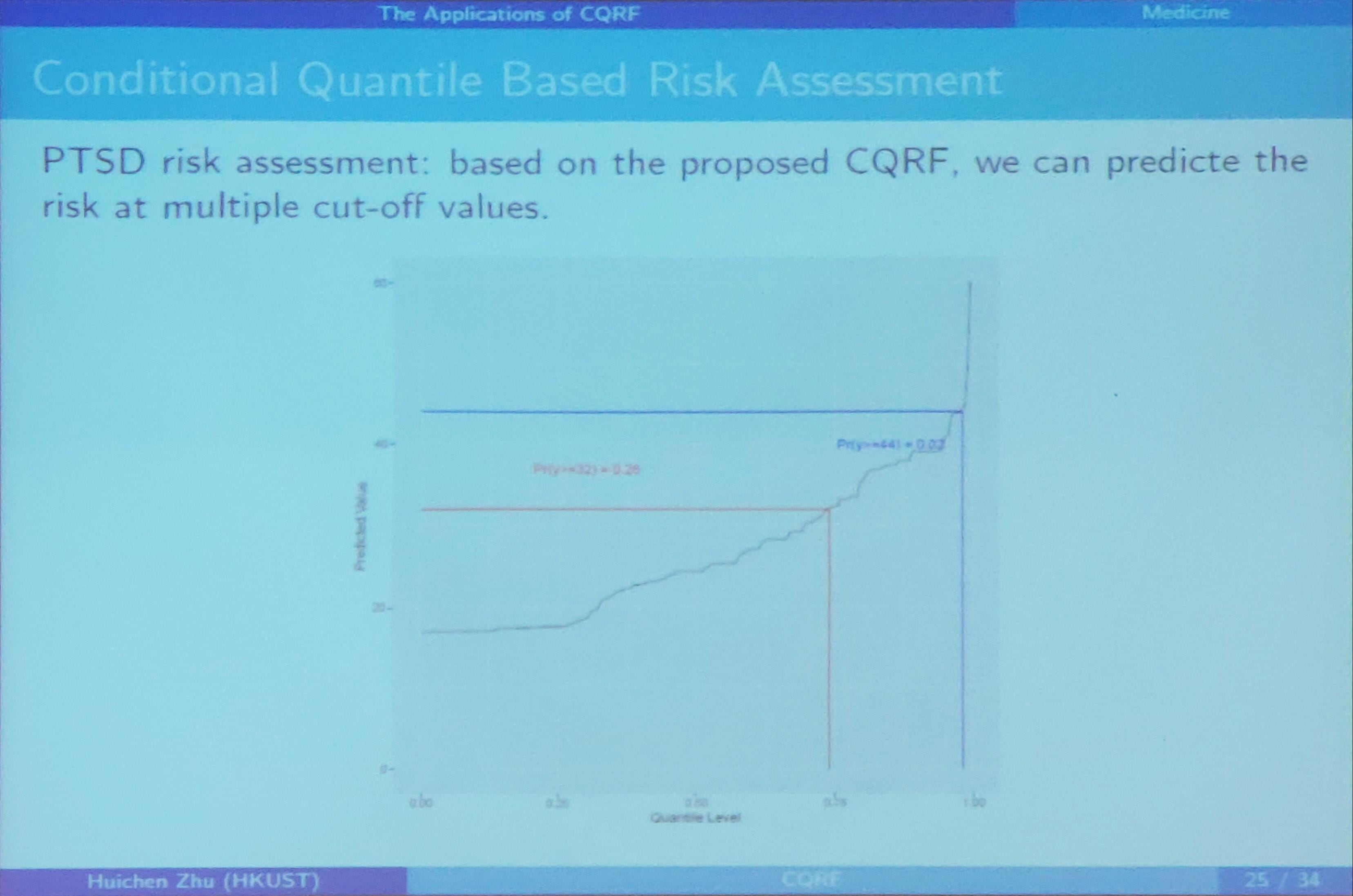
Conditional Quantile Based Risk Assessment

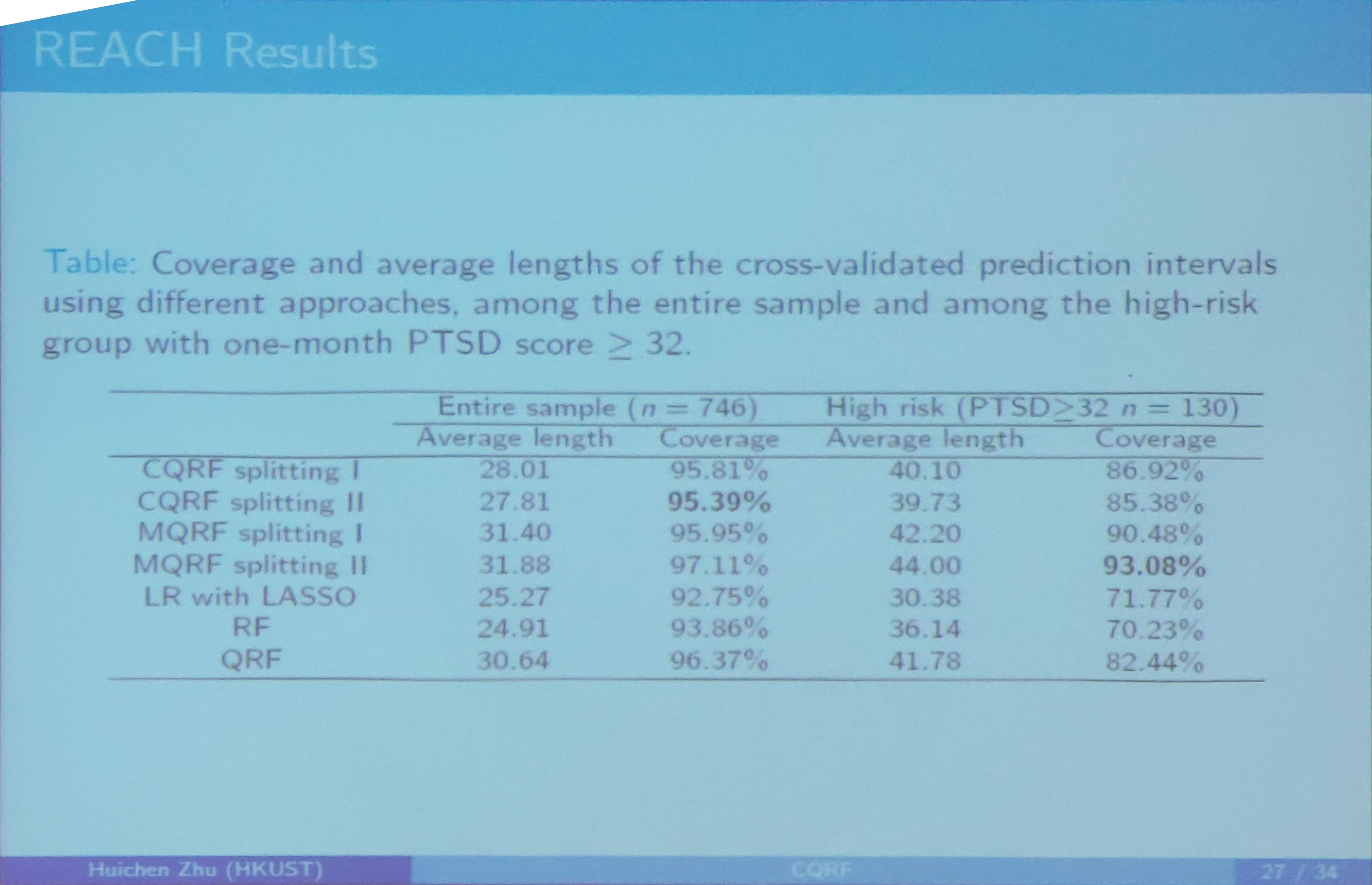
REACH Result

Compare prediction accuracy among the following approaches

• Marginal Quantile RF: treating both $(z, x)$ as splitting variables
• Linear Regression with LASSO: using linear regression, regress one-month PTSD against $(x, z)$, and use a LASSO penalty to select the predictors.
• Random Forest: build the classical mean based random forest using both $x$ and $z$ as splitting variables. The prediction interval is constructed based on predicted mean and standard deviation
• Quantile Regression Forest: The prediction interval is based on the empirical distribution.

Conclusion for CQRF

a robust and efficient approach for improving the screening and intervention strategies.

• it complements the mean-based approaches and fully takes the population heterogeneity into account.
• the use of conditional quantile regression at each split also provides a convenient way to incorporate domain knowledge to improve prediction accuracy (why bother use $\beta$, directly input $x, z$ into the forest can also combine the domain knowledge)
• incorporate with treatment assignment allow to directly estimate individualized treatment effect for precision care (?? not say related materials)

Ongoing work and future extensions

• explore its applications in gene-environment interactions, and develop a new splitting criterion for large-scale but highly correlated genetics data
• the approach could be extended to a longitudinal outcome, where PTSD score might be measured at different time points. (any details?!)
• the approach could be extended to a survival outcome (any details)

Q & A

Here are the questions and the speaker’s answers, only keywords are recorded.

• Q: How to deal with missing data?
• A: For missed response, directly delete. For covariates, surrogate.
• Q: What if misspecified model in the form?
• A: The non-parametric actually is quite flexible.
• Q: Theories about variable selection, such as some accuracy bounds?
• A: No.
• Q: Compared with other machine methods?
• A: Not enough.