ABC for Socks
Posted on
This post is based on Prof. Robert’s slides on JSM 2019 and an intuitive blog from Rasmus Bååth.
The central concept of Bayesian inference would be
\[\pi(\theta\mid x^{\obs}) \propto \pi(\theta)\cdot L(\theta\mid x^{\obs})\,.\]Exploration of posterior $\pi(\theta\mid x^\obs)$ may require to produce sample
\[\theta_1,\ldots,\theta_T\]distributed from $\pi(\theta\mid x^\obs)$. MCMC is the workhorse of practical Bayesian analysis, except when product
\[\pi(\theta)\cdot L(\theta\mid x^\obs)\]well-defined but numerically unavailable or too costly to compute.
ABC stands for approximate (wrong likelihood) Bayesian (right prior) computation (producing a parameter sample).
When likelihood $f(x\mid \theta)$ not in closed form, we can use the following likelihood-free rejection technique.
ABC-AR algorithm
For an observation $x^\obs\sim f(x\mid \theta)$, under the prior $\pi(\theta)$, keep jointly simulating
\[\theta'\sim \pi(\theta), z\sim f(z\mid \theta')\]until the auxiliary variable $z$ is equal to the observed value,
\[z = x^\obs\,.\]Example: Socks
Draw 11 socks out of $m$ socks made of $f$ orphans and $g$ pairs, i.e., $f+2g=m$, number $k$ of socks from the orphan group is hypergeometric $H(11, m, f)$ and the probability to observe 11 orphan socks total is
\[\sum_{k=0}^{11}\frac{\binom{f}{k}\binom{2g}{11-k}}{\binom{m}{11}}\cdot \frac{2^{11-k}\binom{g}{11-k}}{\binom{2g}{11-k}}\,.\]Prior Sock Distributions
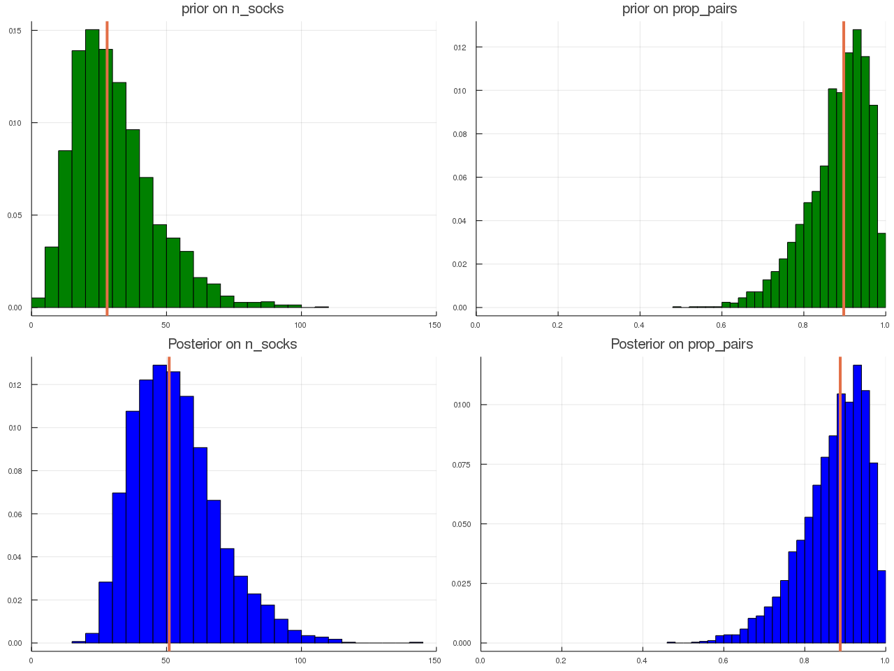
We knows that $n_{\text{socks}}$ must be positive and discrete. A reasonable choice would perhaps be to use a Poisson distribution as a prior, but the Poisson is problematic in that both its mean and its variance is set by the same parameter. Instead we could use the more flexible cousin to the Poisson, the negative binomial. More specifically,
\[n_{\text{socks}} \sim \text{Negative-Binomial}(30, 15)\,.\]Put a prior over the proportion of socks that come in pairs, that is
\[2n_{\text{pairs}} / n_{\text{socks}} \sim \text{Beta}(15, 2)\,.\]Implementations
using Distributions
using Plots
using StatsBase

function sim_socks(nrep = 1000, n_picked = 11)
    # prior of n_socks
    prior_mu = 30
    prior_sd = 15
    prior_p = 1 - prior_mu / prior_sd^2
    prior_size = prior_mu * (1 - prior_p) / prior_p
    prior_n_socks = NegativeBinomial(prior_size, 1-prior_p)
    # prior on the proportion
    prior_prop_pairs = Beta(15, 2)

    # simulate
    res = zeros(nrep, 6)
    for i = 1:nrep
        n_socks = rand(prior_n_socks)
        prop_pairs = rand(prior_prop_pairs)
        n_pairs = round(Int, n_socks * prop_pairs / 2)
        n_orphan = n_socks - n_pairs * 2
        socks = vcat(collect(1:n_orphan+n_pairs), collect(1:n_pairs))
        picked_socks = sample(socks, min(n_picked, n_socks))
        if length(picked_socks) == 0
            res[i, :] = [0, 0, n_socks, n_pairs, n_orphan, prop_pairs]
        else
            freq_socks = values(countmap(picked_socks))
            res[i, :] = [sum(freq_socks .== 1), sum(freq_socks .== 2), n_socks, n_pairs, n_orphan, prop_pairs]
        end
    end
    return res
end

res = sim_socks(100000)
idx = (res[:, 1] .== 11) .& (res[:, 2] .== 0)
post_samples = res[idx, :]
The parametrization of NegativeBinomial() in Julia follows Wolfram’s definition, which is different from Wiki’s (R adopts this definition), but actually just replace the success probability $p$ with $1-p$ in Wiki’s definition.