Exponential Twisting in Importance Sampling
Posted on (Update: )
This note is based on Ma, J., Du, K., & Gu, G. (2019). An efficient exponential twisting importance sampling technique for pricing financial derivatives. Communications in Statistics - Theory and Methods, 48(2), 203–219.
Consider the problem of estimating
\[\alpha = E_f(G(X)) = \int G(x)f(x)dx\]where $X$ is a random vector of $\IR^N$ with probability density $f$, and $G$ is a function from $\IR^N$ to $\IR$.
The usual MC estimate is
\[\alpha_f = \frac 1n\sum_{i=1}^nG(X_i)\,,\]where $X_i$ independently draws from $f$.
If there is another probability density $g$, then alternatively
\[\alpha = E_g\left[G(X)\frac{f(X)}{g(X)}\right]\,.\]In the framework of Gaussian vector, the ordinal density $f(x)$ is
\[f(x) = (2\pi)^{-N/2}\exp\left(-\frac 12\Vert x\Vert^2\right)\,,\]where $x = (x_1,\ldots,x_N)$.
Some research is mainly on adding a drift vector $\mu=(\mu_1,\ldots,\mu_N)$ and the new corresponding density is
\[g_\mu(x) = (2\pi)^{-N/2}\exp\left(-\frac 12\Vert x-\mu\Vert^2\right)\,,\]then the key problem is how to achieve the following minimum
\[\min_\mu E_f\left[ G^2(X) \frac{f(X)}{g_\mu(X)} \right]\,,\]since
\[E_g\left[ \left(G(X)\frac{f(X)}{g(X)}\right)^2 \right] =E_f\left[G(X)^2 \frac{f(X)}{g(X)} \right]\,,\]and the importance sampling estimate is an unbiased estimate.
Consider a ratio estimator
\[\delta_h^n = \sum_{i=1}^nw_ih(x_i)/\sum_{i=1}^nw_i\,,\]where $X_i\sim g(y)$ and $g$ is a candidate distribution for target $f$. The $w_i$’s are realizations of random variables $W_i$ such that $\E[W_i\mid X_i=x] = \kappa f(x)/g(x)$, $\kappa$ being an arbitrary constant (that corresponds to the lack of normalizing constants in $f$ and $g$)but $f$ and $g$ are already supposed to be density functions. Denote
\[S_h^n = \sum_{i=1}^n W_ih(X_i), S_1^n=\sum_{i=1}^nW_i\,.\]Then the asymptotic variance of $\delta_h^n$ is
\[\var(\delta_h^n) = \frac{1}{n^2\kappa^2}(\var(S_h^n)-2\E_f[h]\cov(S_h^n, S_1^n) + (\E_f[h])^2\var(S_1^n))\,.\]
The key step in the proof is the approximation of the variance of a ratio $X/Y$ by the delta method.
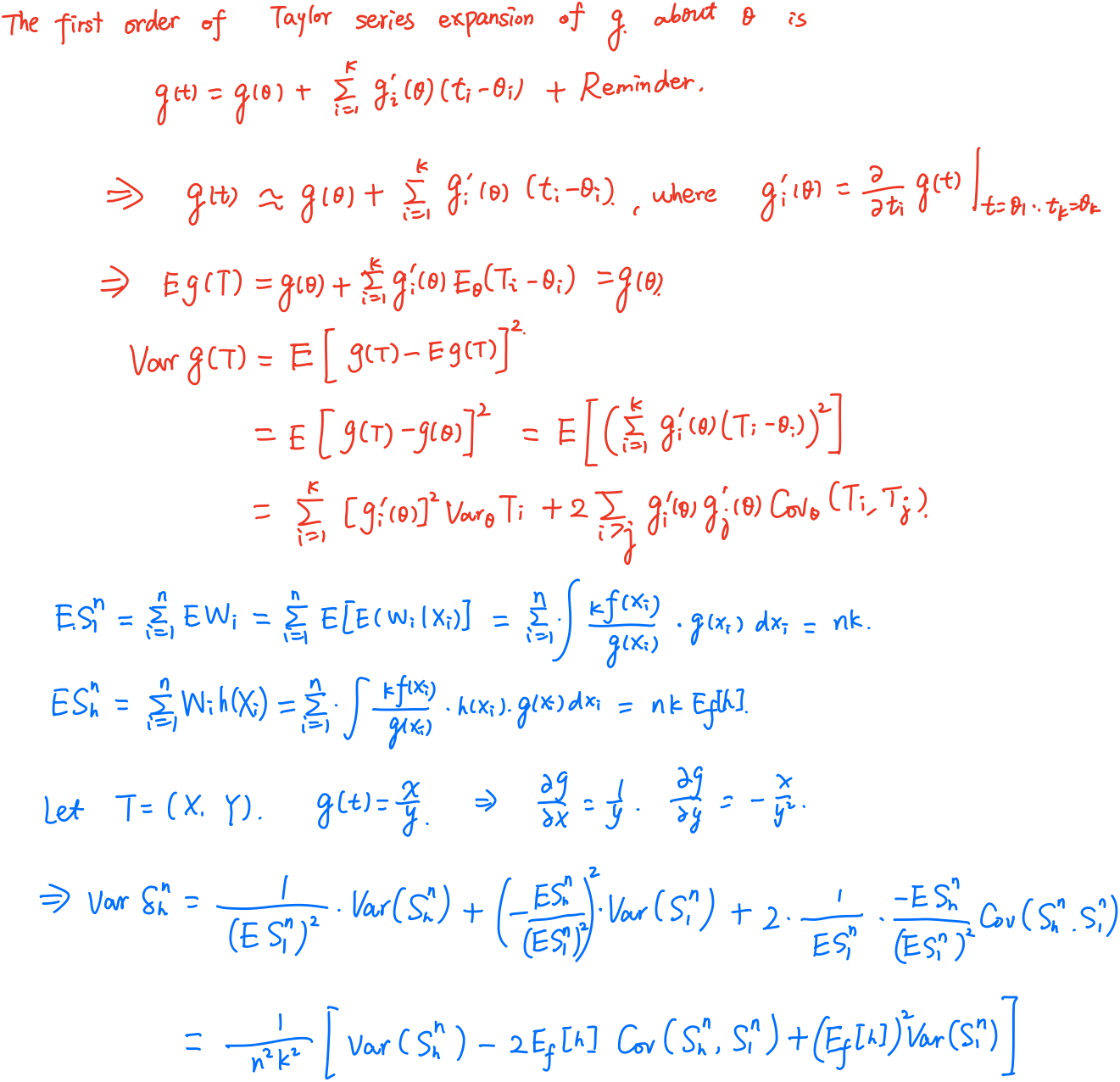
Let $T_1,\ldots, T_k$ be random variables with means $\theta_1,\ldots,\theta_k$. Then
\[\var_\theta(g(T))\approx \sum_{i=1}^k[g_i'(\theta)]^2\var_\theta T_i+2\sum_{i > j}g_i'(\theta)g_j'(\theta)\cov_\theta(T_i,T_j)\,.\]
Further calculation and approximation give Liu (1996)’s ‘rule of thumb’: the effective sample size resulting from an importance sampling procedure is approximately
\[\frac{N}{1+\var_g(w(X))}\,.\]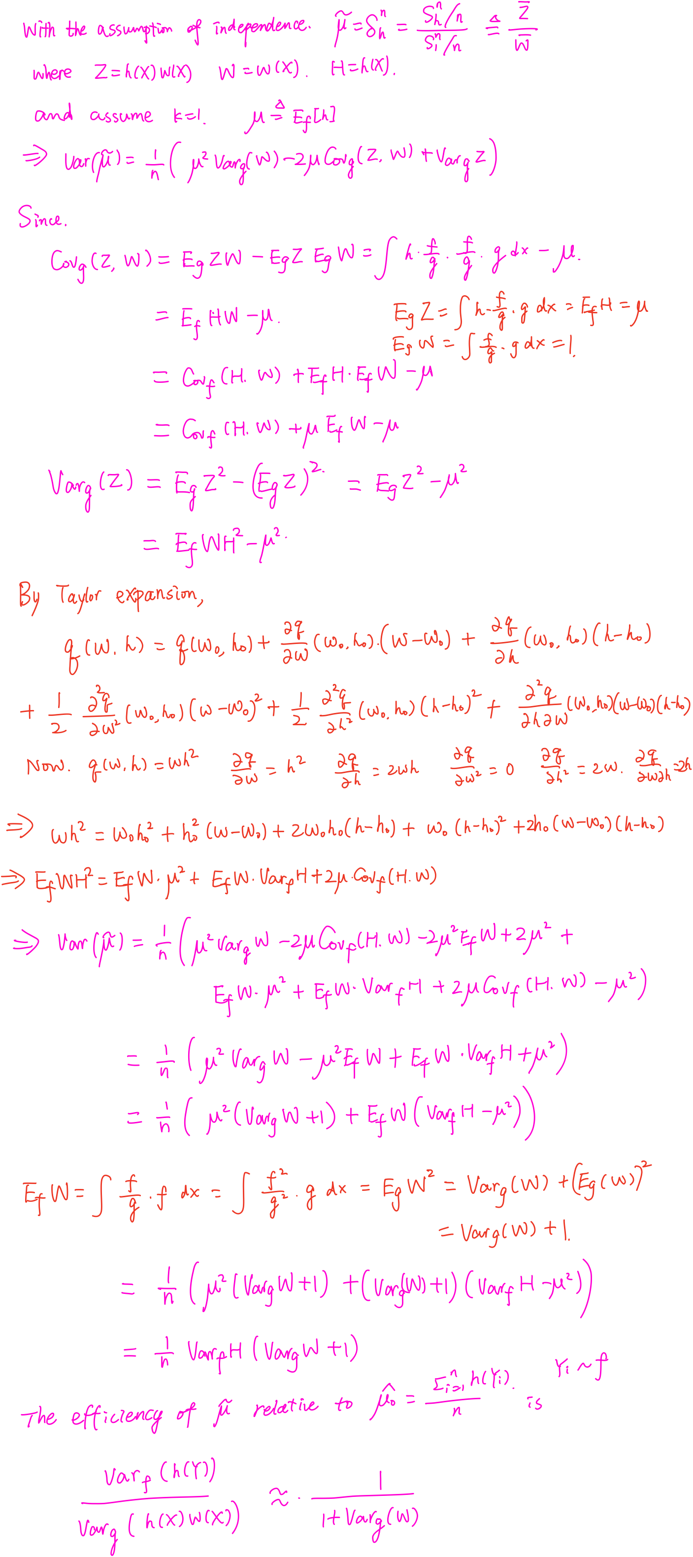
For a cumulative distribution function $F$ on $\IR^N$, define the cumulant generating function of $F$,
\[\psi(\vartheta) = \log\left(\int_{\IR^N}e^{\psi_\vartheta(x)}dF(x)\right)=\log E[e^{\phi_\vartheta}(X)]\,,\]where $\phi_\vartheta(x)$ is called exponential twisting function, if $\phi_\vartheta(x)$ is chosen to satisfy $\psi(\vartheta) < \infty$.
For each twisting function $\phi_\vartheta(x)$, set
\[F_{\phi_\vartheta}(x) = \int_{-\infty}^{x_1}\cdots\int_{-\infty}^{x_N}e^{\phi_\vartheta(y)-\psi(\vartheta)}dF(y)\,.\]It can be showed that $F_{\phi_\vartheta}(x)$ is a probability distribution and $\{F_{\phi_\vartheta},\vartheta\}$ form an exponential family of distributions. The transformation from $F$ to $F_{\phi_\vartheta}$ is called Exponential Twisting or Exponential change of measure.
If $F$ has a density $f$, then $F_{\phi_\vartheta}$ has density
\[f_{\phi_\vartheta}(x) = e^{\phi_\vartheta(x)-\psi(\vartheta)}f(x) = \frac{f(x)}{W(x)}\,,\]here the weighted function $W(x)=e^{-\phi_\vartheta(x)+\psi(\vartheta)}$, so $f(x)=W(x)f_{\phi_\vartheta}(x)$.
The aim is to compute the expectation $V=E[G(X)]$. Using exponential twisting function $\phi_\vartheta(x)$, we have
\[V=E[G(X)]=E_\vartheta[G(X)W(X)]\]and the second moment of $G(X)W(X)$ under $P_{\phi_\vartheta}$
\[E_\vartheta[G^2(X)W^2(X)]=E[G^2(X)W(X)]\,.\]By the Cauchy-Schwarz inequality,
\[E[G^2(X)W(X)] = E[G^2(X)e^{-\phi_\vartheta}(X)]\cdot E[e^{\phi_\vartheta}(X)]\ge E^2[G(X)] = V^2\,.\]It follows that
\[\Var_\vartheta[G(X)W(X)] = E_\vartheta[G^2(X)W^2(X)] - E_\vartheta^2[G(X)W(X)] =E_\vartheta[G^2(X)W^2(X)]-V^2\,.\]In order to achieve the optimal situation, we have
\[\log(G(X))=\varphi_\vartheta(X)\,,\]but in this case, $\psi(\vartheta)=\log(E[G(X)])$ = \log(V) cannot be computed analytically, as $V$ is unknown.
Apply Taylor Expansion for $\log(G(X))$,
\[\log G(X) = \log G(X_1^0,\ldots,X_N^0) + \sum_{i=1}^N(X_i-X_i^0)\frac{\partial \log(G(X_1^0,X_2^0,\ldots,X_N^0))}{\partial X_i} + \\\frac{1}{2!}\sum_{i,j=1}^N(X_i-X_i^0)(X_j-X_j^0)\frac{\partial^2\log(G(X_1^0,X_2^0,\ldots,X_N^0))}{\partial X_i\partial X_j}+O(\rho^3)\,,\]where $\rho=\sqrt{\sum_{i=1}^N(X_i-X_{i0})^2}$.
Write
\[\log(G(X)) = \beta_0 + \sum_{i=1}^N\beta_iX_i + \sum_{i=1}^N\sum_{j=i}^N\beta_{ij}X_iX_j+\varepsilon\,.\]In order to avoid overfitting and simplify the least square regression, remove the cross terms,
\[\phi_\vartheta(x)=\beta_0 + \sum_{i=1}^N\beta_ix_i + \sum_{i=1}^N\beta_{ii}x_i^2 = \beta_0 + \beta' x + x' B x\]