Likelihood-free inference by ratio estimation
Posted on
This note is for Thomas, O., Dutta, R., Corander, J., Kaski, S., & Gutmann, M. U. (2016). Likelihood-free inference by ratio estimation. ArXiv:1611.10242 [Stat]., and I got this paper from Xi’an’s blog.
Abstract
Problem
parametric statistical inference when likelihood computations are prohibitively expensive but sampling from the model is possible.
Several likelihood-free methods
- synthetic likelihood approach: infers the parameters by modelling summary statistics of the data by a Gaussian probability distribution.
- approximate Bayesian computation: the inference is performed by identifying parameter values for which the summary statistics of the simulated data are close to those of the observed data
- synthetic likelihood is easier to use as no measure of “closeness” is required but the Gaussianity assumption is often limiting.
- both of them require judiciously chosen summary statistics.
The paper
easy to use as synthetic likelihood but not are restricted in its assumptions, and that, in a natural way, enables automatic selection of relevant summary statistic from a large set of candidates.
basic idea: frame the problem of estimating the posterior as a problem of estimating the ratio between the data generating distribution and the marginal distribution.
it can be solved by logistic regression, and including regularising penalty terms enables automatic selection of the summary statistics relevant to the inference task.
illustrate the general theory on canonical examples and employ it to perform inference for challenging stochastic nonlinear dynamical systems and high-dimensional summary statistics.
Introduction
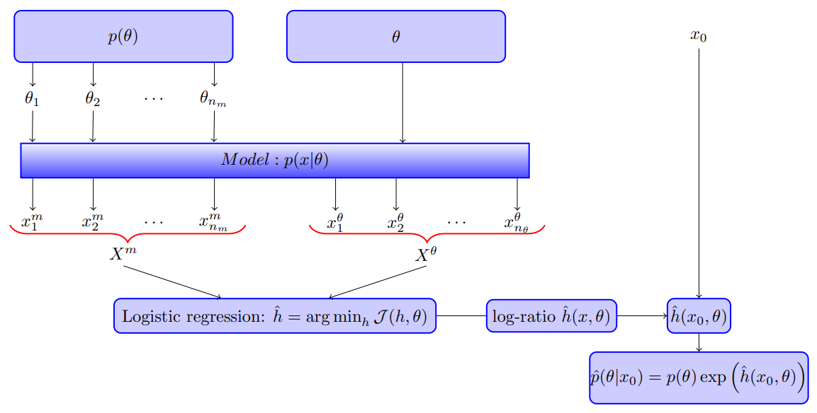
Frame the original problem of estimating the posterior as a problem of estimating the ratio $r(x,\theta)$ between the data generating pdf $p(x\mid \theta)$ and the marginal distribution $p(x)$, in the context of a Bayesian belief update
\[r(x,\theta) = \frac{p(x\mid \theta)}{p(x)}\,.\]An estimate $\hat r(x,\theta)$ for the ratio implies an estimate $\hat p(\theta\mid x_0)$ for the posterior,
\[\hat p(\theta\mid x_0)=p(\theta)\hat r(x_0,\theta)\,.\]In addition, the estimated ratio also yields an estimate $\hat L(\theta)$ of the likelihood function,
\[\hat L(\theta)\propto \hat r(x_0,\theta)\,,\]as the denominator $p(x)$ in the ratio does not depend on $\theta$.
Posterior estimation by logistic regression
Working with a simulator-based model,
- generate data from the pdf $p(x,\theta)$ in the numerator of the ration $r(x,\theta)$, $X^\theta=\{x_i^\theta\}_{i=1}^{n_\theta}$ be such a set with $n_\theta$ independent samples generated with a fixed value of $\theta$.
- generate data from the marginal pdf $p(x)$ in the denominator of the ratio, $X^m=\{x_i^m\}_{i=1}^{n_m}$ be such a set with $n_m$ independent samples.
As the marginal $p(x)$ is obtained by integrating out $\theta$, the samples can be obtained by first sampling from the joint distribution of $(x,\theta)$ and then ignoring the sampled parameters,
\[\theta_i\sim p(\theta)\,,\qquad x_i^m\sim p(x\mid \theta_i)\,.\]Formulate a classification problem where we aim to determine whether some data $x$ were sampled from $p(x\mid \theta)$ or from $p(x)$.
\[P(x\in X^\theta;h) = \frac{1}{1+\nu \exp(-h(x))}\,,\]with $\nu=n_m/n_\theta$ compensating for unequal class sizes.
A suitable function $h$ is typically found by minimising the loss function (equivalent to maximizing the log-likelihood) $\cJ$ on the training data $X^\theta$ and $X^m$,
\[\cJ(h,\theta)=\frac{1}{n_\theta+n_m}\left\{ \sum_{i=1}^{n_\theta}\log[1+\nu \exp(-h(x_i^\theta))] + \sum_{i=1}^{n_m}\log[1+\exp(h(x_i^m))/\nu] \right\}\]The paper shows that for large $n_m$ and $n_\theta$, the minimising function $h^*$ is given by the log-ratio between $p(x\mid \theta)$ and $p(x)$, that is
\[h^*(x,\theta)=\log r(x,\theta)\,.\]$p(x)$ and $p(x\mid \theta)$ is separable?_{:comment}
For finite sample size $n_m$ and $n_\theta$, the minimizing function $\hat h$,
\begin{equation} \hat h=\arg\min_h\cJ(h,\theta)\,.\label{eq:h} \end{equation}
Exponential family approximation
Restrict the search in \eqref{eq:h} to functions $h$ that are members of the family spanned by $b$ summary statistics $\psi_i(x)$, each mapping data $x\in\cX$ to $\IR$,
\[h(x) = \sum_{i=1}^b\beta_i\psi_i(x)=\beta^T\psi(x)\,,\]with $\beta_i\in \IR, \beta=(\beta_1,\ldots,\beta_b)$, and $\psi(x)=(\psi_1(x),\ldots,\psi_b(x))$. This corresponds to performing logistic regression with a linear basis expansion. Then the estimation of the ratio $r(x,\theta)$ boils down to the estimation of the coefficients $\beta_i$. This is done by minimising $J(\beta,\theta)=\cJ(\beta^T\psi,\theta)$ w.r.t. $\beta$.
A synthetic likelihood approximation with summary statistics $\phi$ corresponds to an exponential family approximation where the summary statistics $\psi$ are the individual $\phi_k$, all pairwise combinations $\phi_k\phi_{k’}, k\ge k’$, and a constant. While in the synthetic likelihood approach, the weights of the summary statistics are determined by the man and covariance matrix of $\phi$, but here they are determined by the solution of the optimisation problem.
Data-driven selection of summary statistics
Work with a large list of candidate summary statistics and automatically select the relevant ones in a data-driven manner.
Use the $L_1$ norm of the coefficients as penalty term, like in lasso regression,
\[\hat\beta(\theta,\lambda)=\arg\min_{\beta\in\IR^b}J(\beta,\theta)+\lambda\sum_{i=1}^b\vert \beta_i\vert\,.\]Choose $\lambda$ by minimising the prediction risk $\cR(\lambda)$,
\[\cR(\lambda) = \frac{1}{n_\theta+n_m}\left\{ \sum_{i=1}^{n_\theta}\1_{\Pi_\lambda(x_i^\theta) < 0.5} + \sum_{i=1}^{n_m}\1_{\Pi_\lambda(x_i^m) > 0.5} \right\}\]estimated by ten-fold cross-validation, where $\Pi_\lambda(x)=P(x\in X^\theta; h(x)=\hat\beta(\theta,\lambda)^T\psi(x))$
Validation on canonical low-dimensional problems
TODO: implement by myself.
Discussion
- the approach for posterior estimation with generative models mirrors the approach of Gutmann and Hyvärinen (2012) for the estimation of unnormalised models. The main difference is that, here classify two simulated data sets while Gutmann and Hyvärinen (2012) classified between the observed data and simulated reference data.
- the method requires that several samples from the model generated for the estimation of the posterior at any parameter value. There are several ways to reduce it.
- a key feature of the proposed approach is the automated selection and combination of summary statistics from a large pool of candidates.
- the method has not been fully investigated in high-dimensional case.
- more general regression models and other loss functions.