A Optimal Control Approach for Deep Learning

Posted on Jul 19, 2019

Tags: Deep Learning, Optimal Control

This note is based on Li, Q., & Hao, S. (2018). An Optimal Control Approach to Deep Learning and Applications to Discrete-Weight Neural Networks. ArXiv:1803.01299 [Cs].

The Optimal Control Viewpoint

• $T\in \bbZ_+$: the number of layers
• ${x_{s,0}\in\bbR^{d_0}:s=0,\ldots,S}$: a collection of fixed inputs
• $S\in \bbZ_+$: sample size

Consider the dynamical system

\[x_{s,t+1} = f_t(x_{s,t},\theta_t),\quad t=0,1,\ldots,T-1\,,\]

(represent affine transformation and nonlinear activation in a layer?)

the goal of training a neural network is to adjust the weights $\theta = {\theta_t:t=0,\ldots,T-1}$ so as to minimize some loss function that measures the difference between the final network output $x_{s,T}$ and some true targets $y_s$ of $x_{s,0}$.

Define a family of real-valued function $\Phi_s:\bbR^{d_T}\rightarrow \bbR$ acting on $x_{s,T}$ ($y_s$ are absorbed into the definition of $\Phi_s$).

In addition, consider some regularization terms for each layer $L_t:\bbR^{d_t}\times\Theta_t\rightarrow \bbR$ that has to be simultaneously minimized. Here slightly more general case regularize the sate at each layer, not only trainable parameters (!!).

In summary,

\[\min_{\theta\in\Theta}\;J(\theta) = \frac 1S\sum_{s=1}^S\Phi_s(x_s,T) + \frac 1S\sum_{s=1}^S\sum_{t=0}^{T-1}L_t(x_{s,t}, \theta_t)\]

subject to

\[x_{s,t+1} = f_t(x_{s,t}, \theta_t), t=0,\ldots,T-1,s\in[S]\]

where

• $\Theta={\Theta_0\times\cdots\times \Theta_{T-1}}$
• $[S]={1,\ldots,S}$.

The Pontryagain’s Maximum Principle

Maximum principles of the Pontryagain type usually consist of necessary conditions for optimality in the form of the maximization of a certain Hamiltonian function.

Distinguishing feature: does not assume differentiability (or even continuity) of $f_t$ w.r.t. $\theta$

Thus, the optimality condition and the algorithms based on it need not rely on gradient-descent type updates.

Define the Hamiltonian function $H_t:\bbR^{d_t}\times \bbR^{d_{t+1}}\times \Theta_t\rightarrow\bbR$ by

\[H_t(x,p,\theta) = pf_t(x,\theta) - \frac 1SL_t(x,\theta)\,.\]

Let $\theta^*$ be a solution. The necessary conditions are:

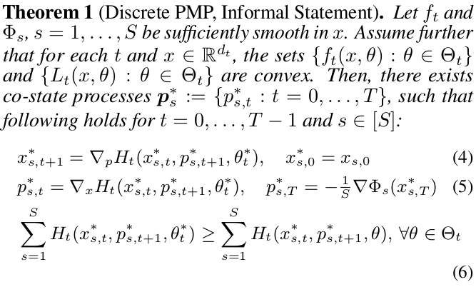
• eq (4): the forward propagation equation
• eq (5): the evolution of the co-state $p_s^*$
• eq (6): an optimal solution $\theta^*$ must globally maximize the summed Hamiltonian for each layer $t=0,\ldots,T-1$

The Convexity Assumption

Convexity of ${f_t(x,\theta):\theta\in\Theta_t}$

Two types of layers:

• non-trainable (non-linear activation function): trivially convex since singleton
• trainable:
  • $f_t$ is usually (?) affine in $\theta$: fully connected layers, convolution layers and batch normalization layers
  • as long as the admissable set $\Theta_t$ is convex.
  • residual networks also satisfy the convexity constraints if one introduces auxillary variables.
  • if $\Theta_t$ is not convex, generally PMP not constitute necessary conditions.

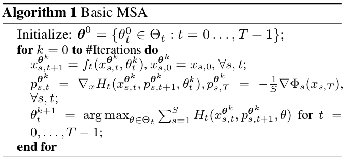
The Method of Successive Approximations

Algorithm based on the maximum principle: how to find the solution.

Each of eq. (4)-(6) represent a manifold in solution space consisting of all possible $\theta,{x_s,s\in[S]}$ and ${p_s,s\in [S]}$, and the intersection of these three manifolds must contain an optimal solution, if one exists.

Thus, an iterative projection method that successively projects a guessed solution onto each of the manifolds.

An Error Estimate for the MSA

(the discontinuity not account for the continuity of $\Theta_t$??)

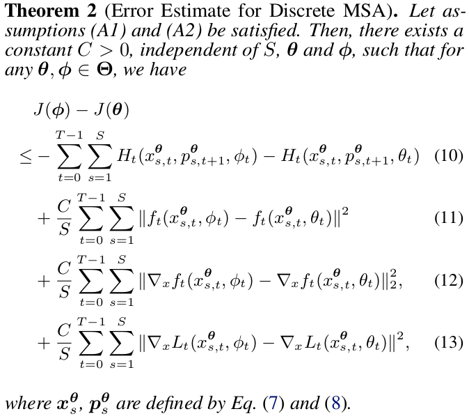
Intuitively, the Hamiltonian maximization step is generally the right direction, but we will incur nonnegative penalty terms when changing the parameters from $\theta$ to $\phi$.

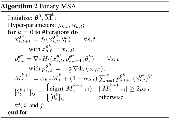
Neural Networks with Discrete Weights

Main strength: not gradient-descent, thus useful when the trainable parameters only take values in a discrete set.

• binary networks: weights are restricted to ${-1,+1}$
• ternary networks: ${-1,+1,0}$

Binary networks

for simplicity only the fully connected case

Ternary networks

goal: explore the sparsification of the network

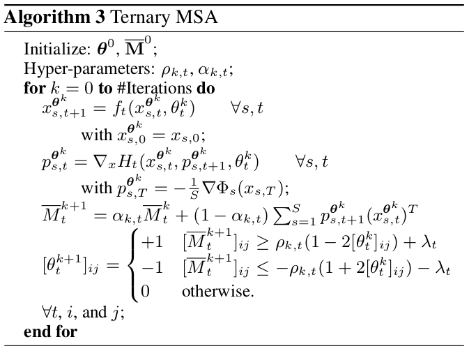
results: similar performance but high degrees of sparsity.

Discussion and Related Work

1. convexity assumption are justified for conventional neural networks, but not necessarily so for all neural networks
2. the usual BP with gradient-descent can be regarded as a simple modification of MSA with differentiability assumption
3. overfitting in MSA might imply that different way with stochastic gradient based optimization

Literatures:

1. here the optimal control approach is different from prevailing viewpoint of nonlinear programming
2. optimal control and dynamical systems viewpoint has been discussed and dynamical systems based discretization schemes, but most of them have theoretical basis in continuous-time dynamical systems
3. the paper gives a discrete-time formulation
4. the connection between optimal control and deep learning has been qualitative discussed, but fewer works relating optimal control algorithms to training neural networks beyond the classical gradient-descent with back-propagation.
5. binary MSA is competitive, but need to reduce overfitting
6. future work is required to rigorously establish the convergence of these algorithms

Conclusion and Outlook

questions:

• the applicability of the PMP for discrete-weight neural networks, which does not satisfy the convexity assumptions.
• establish the convergence of the algorithms presented.

code is available