Rare Variant Association Testing
Posted on (Update: )
This note is based on
- Wu, M. C., Lee, S., Cai, T., Li, Y., Boehnke, M., & Lin, X. (2011). Rare-Variant Association Testing for Sequencing Data with the Sequence Kernel Association Test. American Journal of Human Genetics, 89(1), 82–93.
- Wang, M. H., Weng, H., Sun, R., Lee, J., Wu, W. K. K., Chong, K. C., & Zee, B. C.-Y. (2017). A Zoom-Focus algorithm (ZFA) to locate the optimal testing region for rare variant association tests. Bioinformatics, 33(15), 2330–2336.
SKAT (Sequencing Kernel Association Test)
- common variants identified by GWASs often explain only a small proportion of trait heritability
- rare genetic variants, alleles with a frequency less than 1%-5%, can play roles in influencing complex disease and traits.
- standard methods used to test for association with single common genetic variants are underpowered for rare variants unless sample sizes or effect sizes are very large
A logical alternative approach: burden tests
- assess the cumulative effects of multiple variants in a genomic region.
- limitation: implicitly assume that all rare variants influence the phenotype in the same direction and with the same magnitude of effect, but most variants (common or rare) within a sequenced region to have little or no effect on phenotype, whereas some variants are protective and others deleterious, and the magnitude of each variant’s effect is likely to vary.
non-burden-based test: C-alpha test
- robust to the direction and magnitude of effect
- not allow for easy covariate adjustment
- also use permutation
SKAT: tests for association between variants in a region (both common and rare) and a dichotomous (e.g. case-control) or continuous phenotype while adjusting for covariates.
- a multiple regression model to directly regress the phenotype on genetic variants in a region and on covariates
- kernel association test to test the regression coefficients of the variants by using a variance-component score test in a mixed-model framework by accounting for rare variants
- allowance for epistatic variant effects.
epistasis(上位效应)
 来源:
来源:Assume $n$ subjects are sequenced in a region with $p$ variant sites observed.
For the $i$-th subject,
- $y_i$: the phenotype variable
- $X_i=(X_{i1},\ldots,X_{im})$: the covariates, might include age, gender, and top principal components of genetic variation for controlling population stratification.
- $G_i=(G_{i1},\ldots,G_{ip})$: the genotype for the $p$-variants within the region.
Consider the linear model
\[y_i=\alpha_0 + \alpha'X_i + \beta'G_i + \varepsilon_i\]when the phenotypes are continuous traits, and the logistic model
\[\logit P(y_i=1) = \alpha_0 + \alpha'X_i + \beta'G_i\]when the phenotypes are dichotomous.
Evaluating whether the gene variants influence the phenotype, adjusting for covariates, corresponding to testing the null hypothesis $H_0:\beta=0$.
The standard p-DF (?? TODO) likelihood ratio test has little power, especially for rare variants. SKAT tests $H_0$ by assuming each $\beta_j$ follows an arbitrary distribution with a mean of zero and a variance of $w_j\tau$, where $\tau$ is a variance component and $w_j$ is a pre-specified weight for variant $j$.
Then $H_0:\beta=0$ is equivalent to testing $H_0:\tau = 0$, which can be tested with a variance-component score test in the corresponding mixed model; this is known to be a locally most powerful test.
Specifically, the variance-component score statistic is
\[Q = (y - \hat \mu)'K (y - \hat\mu)\,,\]where $K=GWG’$, $\hat \mu$ is the predicted mean of $y$ under $H_0$.
- $G$: an $n\times p$ matrix with the $(i, j)$-th element being the genotype of variant $j$ of subject $i$
- $W = \diag(w_1,\ldots,w_p)$ contains the weights of the $p$ variants
And $K(G_i, G_{i’})=\sum_{j=1}^pw_jG_{ij}G_{i’j}$ measures the genetic similarity between subject $i$ and $i’$ in the region via the $p$ markers.
In practice, propose $\sqrt{w_j}=\mathrm{Beta}(\mathrm{MAF}_j;a_1,a_2)$
- $0 < a_1 \le 1$ and $a_2 \ge 1$: increasing the weight of rarer variants and decreasing the weight of common weights, a smaller $a_1$ results in more strongly increasing the weight of rarer variants
- $a_1 = a_2 = 1$, reduce to Uniform distribution, corresponds to $w_j = 1$
- $a_1=a_2=0.5$ corresponds to $\sqrt{w_j} = \dfrac{1}{\sqrt{\mathrm{MAF}_j(1-\mathrm{MAF}_j)}}$, i.e., the inverse of the variance of the genotype of marker $j$, which puts almost zero weight for MAF > 1% and can be used if one believes only variants with MAF < 1% are likely to be casual. SKAT calculated with this weight is identical to the unweighted SKAT test with the standardized genotypes in the above two equations.
The following figure (with the Julia code for plotting) shows such examples of weights, in which the first row is the pdf, while the second row is the normalized weights as the paper presents.

using Distributions
using Plots
using LaTeXStrings
p1 = plot(0:0.01:1, pdf.(Beta(1, 25), 0:0.01:1),
    label = L"\alpha = 1, \beta = 25",
    ylim = (0, 5), ylabel = "pdf")
plot!(p1, 0:0.01:1, pdf.(Beta(1, 1), 0:0.01:1),
    label = L"\alpha = 1, \beta = 1")
plot!(p1, 0:0.01:1, pdf.(Beta(0.5, 0.5), 0:0.01:1),
    label = L"\alpha = 0.5, \beta = 0.5")
p2 = plot(0:0.01:1, logpdf.(Beta(1, 25), 0:0.01:1),
    label = L"\alpha = 1, \beta = 25", ylabel = "logpdf")
p3 = plot(0:0.001:0.5, pdf.(Beta(1, 25), 0:0.001:0.5) ./ pdf(Beta(1, 25), 1e-3),
    label = L"\alpha = 1, \beta = 25", ylim = (0, 1),
    ylabel = "Weight", xlabel = "MAF")
plot!(p3, 0:0.001:0.5, pdf.(Beta(1, 1), 0:0.001:0.5),
    label = L"\alpha = 1, \beta = 1")
plot!(p3, 0:0.001:0.5, pdf.(Beta(0.5, 0.5), 0:0.001:0.5) ./ pdf(Beta(0.5, 0.5), 1e-3),
    label = L"\alpha = 0.5, \beta = 0.5")
p4 = plot(0:0.001:0.05, pdf.(Beta(1, 25), 0:0.001:0.05) ./ pdf(Beta(1, 25), 1e-3),
    label = L"\alpha = 1, \beta = 25", ylim = (0, 1),
    ylabel = "Weight", xlabel = "MAF")
plot!(p4, 0:0.001:0.05, pdf.(Beta(1, 1), 0:0.001:0.05),
    label = L"\alpha = 1, \beta = 1")
plot!(p4, 0:0.001:0.05, pdf.(Beta(0.5, 0.5), 0:0.001:0.05) ./ pdf(Beta(0.5, 0.5), 1e-3),
    label = L"\alpha = 0.5, \beta = 0.5")
plot(p1, p2, p3, p4)
Under the null hypothesis, $Q$ follows a mixture of chi-square distributions, which can be closely approximated with the computationally efficient Davies method (TODO).
- a special case: dichotomous outcome, no covariates, all $w_j=1$. The SKAT test statistic $Q$ is equivalent to the C-alpha test statistic $T$. So, C-alpha test is a special case of SKAT.
- SKAT under flat weights, the kernel machine regression test, the SSU test, and the C-alpha test are all equivalent and special cases of SKAT.
Relationship between Linear SKAT and Individual Variant Test Statistics
$Q$ is a weighted sum of the individual score test statistics for testing for individual variant effects, that is,
\[Q = \sum_{j=1}^pw_jS_j^2\,,\]where $S_j=g_j’(y-\hat\mu_0), g_j=[G_{1j},\ldots, G_{nj}]’$ is the individual score statistic for testing the marginal effect of the $j$-th marker $H_0:\beta_j=0$.
Accommodating Epistatic Effects and Prior Information under the SKAT
replace $G_i’\beta$ with a more flexible function $f(G_i)$.
ZFA
The challenge of analysing genome sequencing datasets, besides multiple-testing issues arising from high dimensionality, centres on extreme low allele frequencies–classical statistical tests lose power on genetic variants with small variance.
In whole genome or exome sequencing data, over 99% of the variants have minor allele frequency (MAF) below 1%.
MAF in “变异过滤”
参考 生物信息分析:从入门到精(fang)通(qi)第5期 我们的征途是星辰大海 - 知乎.
一个全基因组会产生数百万个变异位点,每个位点都有很多注释信息。但我们的目标往往只有几个或者几十个,所以要尽可能地把不相关的变异过滤掉,找到最可能致病的。
变异过滤 是通过一定的过滤策略,去除与患者表型不太可能相关的变异,并尽可能减少候选变异的数目。常用的过滤策略有
- 数据质量
- 人群频率:不同位点的基因型在人群中的频率是不一样的,不同人群致病变异的携带率也不大一样。一般来说,人群中频率高的突变往往是没有致病性,可以用来过滤,排除常见的良性变异。基因变异程度可根据 次等位基因频率 (minor allele frequency, MAF) 划分,MAF 介于 5%-50% 之间称为常见变异,MAF 介于 1%-5% 之间的为罕见变异。在研究罕见病的致病变异时,应该过滤掉非罕见变异。
- 变异分类
- 疾病知识
- 危害性预测结果
A number of rare variant association tests has been proposed to improved power:
- pulling adjacent variants together and up-weighting the minor allele
- applying a linear mixed model on a certain genomic region (variance component tests)
fixed window
For most rare variant methods, assume a fixed genomic region for testing, such as a gene or a fixed window.
Drawbacks:
- unnecessary noise in a fixed window
- exome data have unknown gene functions
- => need to optimize the collapsing region
Strength: most effective when the true signals display a certain degree of clustering
- not unreasonable as linkage disequilibrium exists among adjacent variants
- variants in the same gene regulatory element would physically cluster in DNA sequences
sliding window
scan statistics: need permutations
- not possible to select window size in an exhaustive manner for whole genome evaluation
- no stand-alone window size optimization for other (?) rare variant association tests.
ZFA
optimize the testing region for any region-based rare variant association test as a wrapper function
- zooming: partition a fixed genomic region by an order of two, search across all partition levels to identify the region with maximum information, evaluated by the smallest association $P$-value of that partition
- focus: refine the region by adding or subtracting adjacent variants near the boundaries.
Materials and Methods
Zoom-Focus algorithm
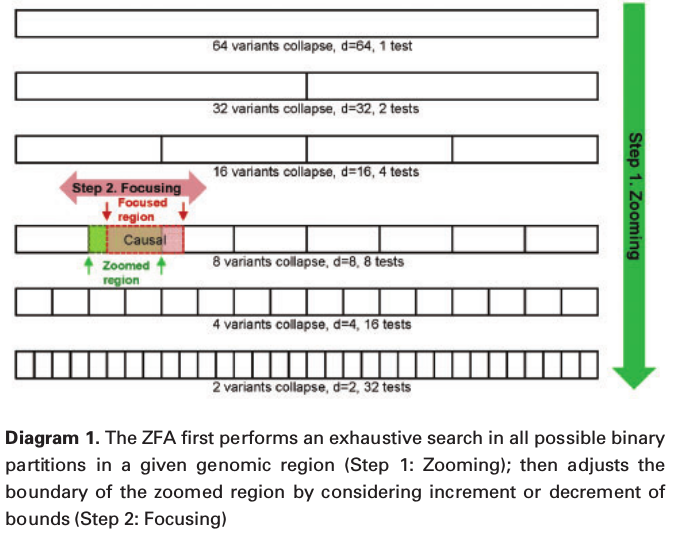
In the above example, $P = 64, r = 4, d = 8, c = 2$. The causal region is $\phi(8, 2)$.
- $P$: total number of variants in a fixed window
- $R$: maximum order of binary partitions for $P$, $R=\arg\max\{r:2^{r-1}<P, r=1,2,\ldots\}$
- $r$: the order of partitions, the corresponding number of regions is $n_r=2^{r-1}$
- $d$: the number of variants in a partitioned region, $d=P/n_r=P/2^{r-1}$
- $c$: the index for the $c$-th partition, $c=1,\ldots,n_r$.
- $\phi(d, c)=\{x_{cj},j=1,\ldots,d\}$: the region that contains variants in a partition size $d$ and index $c$
- $f(\cdot)$ be the Bonferroni corrected $P$-value calculated by rare variant method $F(\cdot)$ measured on region $\phi(d,c)$: $f(d,c)=n_rF[\phi(d,c)]$.
Step 1: Zooming.
\[(\hat d, \hat c) = \arg\min\{f(d,c),r=1,\ldots,R;c=1\text{ to }n_r\}\,.\]the number of tests in a window of $P$ number of variants is
\[T(P) = \sum_{x=0}^{R-1}2^x = 2^R - 1 \approx 2^{\log_2(P)} - = P-1\]therefore, the computational complexity of Zooming is $O(P)$
Step 2: Focusing
Refine the boundaries of $(\hat d,\hat c)$ by extending both lower and upper bounds,
\[\begin{align} LB_f &=\arg\min\{f(LB',UB), LB'=LB+i;i=[-\hat d/2, \hat d/4]\}\\ UB_f &=\arg\min\{f(LB_f,UB'),UB'=UB+i;i=[-\hat d/4, \hat d/2]\} \end{align}\]Then the $P$-value of ZFA on a given window of $P$ variants is:
\[p\text{-value} = (k+P-1)F(LB_f,UB_f)\,,\]where $P-1$ is the number of tests in the zooming step, and $k$ is the number of tests in the Focusing step, $0\le k\le 3/2\hat d$
- $k=0$ when Focusing is not performed
- $k=3/2\hat d$ when Focusing searches the surrounding of both bounds
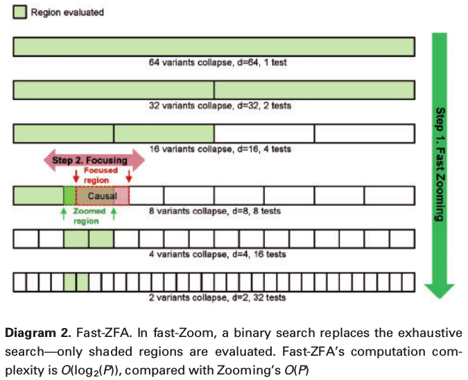
fast-ZOOM
Simulation study design
2000 subjects and 128 rare variants
Real data application
real hypertensive disorder sequence data of the Genetics Analysis Workshop (GAW19)
- 398 hypertensive patients and 1453 healthy controls
- the exome sequence of chromosome 3 is used
- after quality control, 41,788 rare variants remain.
- full ZFA is applied on Chromosome 3 using an initial window size $P=256$
- the chromosome is divided into 163 non-overlapping regions, the remaining 60 variants are grouped as the last window