TreeClone
Posted on (Update: )
Introduction
- Initiated by somatic mutations in a single cell, cancer arises through Darwinian-like natural selection.
- tumorigenesis: the accumulation of subsequent genetic aberrations and the effects of selection over time result in the sequential clonal expansions of cells, finally leading to the development of a genetically aberrant tumor.
- subclones: genetically divergent subpopulations of tumor cells, also known as subclones.
- Deep next generation sequencing (NGS) of bulk tumor DNA samples can examine the evolutionary history of individual tumors by deconvoluting observed genomic data from a tumor into constituent signals corresponding to various subclones and by then reconstructing the relationship of these subclones in a phylogeny.
- phylogentic relationship
- tumor purity
- subclones’ genotypes
- cellular proportions
Numerous methods
- typically based on short reads that are mapped to single nucleotide variants (SNVs)
- many methods based on SNV utilize variant allele fractions (VAFs)–the fractions of alleles (or short reads) at each locus that carry mutations
- most use only marginal SNVs, someone use pairs of proximal SNVs.
- two categories:
- clustering-based (indirectly): first infer SNV clusters based on observed VAFs, and then reconstruct subclonal genotypes based on the clusters. The phylogentic relationship among the subclones can be inferred by imposing hierarchy among the SNV clusters.
- feature-allocation-based (directly): treat subclones as latent features and directly infer subclonal genotypes. Most of them assume that the features (subclones) are conditionally independent and thus are not able to infer the phylogenetic relationship among the subclones. Someone can infer.
The paper
- available data: $T\ge 1$ samples from a single patient
- main inference goal: intra-tumor heterogeneity.
- a novel approach to reconstruct tumor subclones and their corresponding phylogenetic tree based on mutation pairs.
- model tumor heterogeneity based on a representation of a phylogenetic tree of tumor cell subpopulations.
- a prior probability model on such phylogenetic trees induces a dependent prior on the mutation profiles of latent tumor cell subpopulations
Notations:
- $K$ mutation pairs
- $T \ge 1$ samples
- $C$ homogeneous subclones: unknown, one of the model parameters
- $Z$: a $K\times C$ matrix, each column represents a subclone and each row represents a mutation pair.
- $z_{kc}$: a $2\times 2$ matrix that represents the genotypes of the two alleles of the mutation pair.
- $\cT$: a phylogenetic tree, formed by the columns (subclones) of $Z$
- $w_t=(w_{t1},\ldots,w_{tC})$: the cellular proportions of the subclones in sample $t$ where $0 < w_{tc}< 1$ for all $c$ and $\sum_{c=0}^Cw_{tc}=1$.
Using NGS data, infer $\cT,C,Z$ and $w$ based on a simple idea that variant reads can only arise from subclones with variant alleles consistent with an underlying phylogeny.
The paper leverage the power of using mutation pairs over single SNVs to incorporate partial phasing information in our model.
Impose the phylogenetic tree structure in the prior of $Z$ greatly strengthens inference.
- the tree structure improves biological interpretability of the inferred subclones.
- the tree structure improves the identifiability of the problem.
- the tree structure improves the mixing performance of the MCMC simulation.
The proposed model structure versus a traditional use of phylogenetic trees.
- most methods lack assessment of tree uncertainties and report a single tree estimate.
- define a tree with all descendant nodes differing from the parent node by some mutations.
Statistical Model
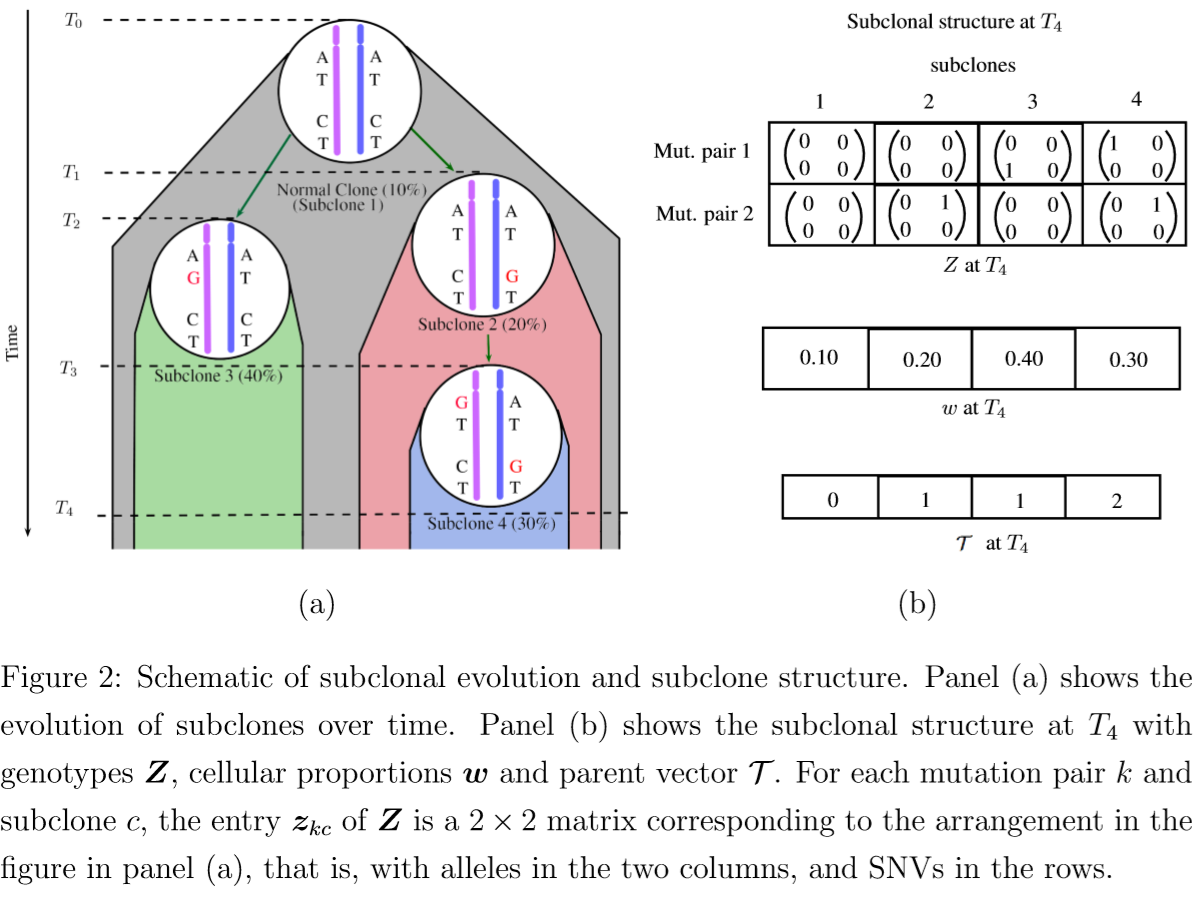
- $\cT$ is a $C$-dimensional parent vector, where $\cT_c=\cT[c]=j$ is the parent of subclone $c$.
where in $z_{kcjr}$, $j$ and $r$ index the two alleles and the two loci.
Assume $z_{kcjr}$ can only take two possible values, with $z_{kcjr}=1$ (or $0$) indicating that the corresponding locus has a mutation (or does not have a mutation) compared to the reference genome.
$w$: a $T\times C$ matrix to record the proportions, $\sum_{c=1}^Cw_{tc}=1$.
$w_{t1}$: the proportion of normal cells contamination in sample $t$.
Sampling model
$N$: a $T\times K$ matrix with $N_{tk}$ representing read depth for mutation pair $k$ in sample $t$.
(the number of times any locus of the mutation pair is covered by sequencing reads)
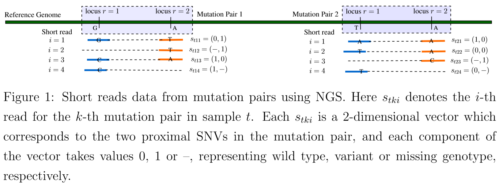
$s_{tki}=(s_{tkir},r=1,2)$: a specific short read, $i=1,2,\ldots,N_{tk}$. Use $s_{tkir}=1$ (or 0) to denote a variant (reference) sequence at the read, compared to the reference genome
- read $i$ may overlap in only one locus, use $s_{tkir}=-$ to represent the missing other sequence on the read.
- reads that do not overlap with either of the two loci are not included in the model as they do not contribute any information about the mutation pair.
$s_{tki}$ can take $G=8$ possible values,
\[s_{tki}\in \{s^{(1)},\ldots,s^{(8)}\} = \{00, 01, 10, 11, -0, -1, 0-, 1-\}\,.\]Assume a multinomial sampling model for the observed read counts
\[(n_{tk1},\ldots,n_{tk8})\mid N_{tk} \sim Mn(N_{tk}; p_{tk1},\ldots, p_{tk8})\]For a short read $s_{tki}$, depending on whether it covers both loci or only one locus, consider these cases
- a read covers both loci (complete read), $s_{tki}\in {s^{(1)},\ldots,s^{(4)}}$
- a read covers the second locus (left missing read): $s_{tki}\in {s^{(5)}, s^{(6)}}$
- a read covers the first locus (right missing read): $s_{tki}\in {s^{(7)}, s^{(8)}}$
(No order? but why here again consider order?)
Let $v_{tki}$ be the probability of observing a short read of type $(i)$. Conditional on cases (i), let $\tilde p_{tkg}$ be the conditional probability.
Express $\tilde p_{tkg}$ in terms of $Z$ and $w$ based on the following generative model (?) in three steps.
Consider a sample $t$. To generate a short read,
- select a subclone $c$ with probability $w_{tc}$
- select with prob. 0.5 one of the two alleles $j=1,2$
- record the read $s^{(g)}$ corresponding to the chosen allele $z_{kcj}=(z_{kcj1},z_{kcj2})$.
the prob. of observing a short read $s^{(g)}$ from subclone characterized by $z_{kc}$ by
\[A(s^{(g)}, z_{kc}) = \sum_{j=1}^2 0.5\times I(s_1^{(g)}=z_{kcj1})I(s_2^{(g)}=z_{kcj2})\,,\]where $I(-=z_{kcjr})\equiv 1$ for missing reads.
the marginal prob. of observing a short read $s^{(g)}$ from the tumor sample $t$ with $C$ subclones with cellular proportions ${w_{tc}}$ as
\[\tilde p_{tkg} = \sum_{c=1}^Cw_{tc}A(s^{(g)},z_{kc}) + w_{t0}\rho_g\,,\]where the last term introduces the notion of a background subclone, indexed as $c=0$ and without biological meaning, to account for noise and artifacts in the NGS data (sequencing errors, mapping errors, etc.)
Prior model
Construct a hierarchical prior model,
- start with $p(C)$: a geometric prior, $p(C)=(1-\alpha)^{C-1}\alpha, C\in{1,2,3,\ldots}$
- a prior on the tree for a given number of nodes: $p(\cT\mid C)\propto \prod_{c=1}^C(1+\eta_c)^{-\beta}$, where $\eta_c$ is the depth of node $c$, or the number of generations between node $c$ and the normal subclone $1$.
- a prior on the subclonal genotypes given the phylogenetic tree $\cT$
- the subclone genotype matrix $Z$ can be thought of as a feature allocation for categorical matrices
- the mutation pairs are the objects, and the subclones are the latent features chosen by the objects (TODO)
- each feature has 10 categories
- given $\cT$ the construction of the subclone genotype matrix needs to introduce dependence across features to respect the assumed phylogeny.
construct a prior for $Z$ based on a generative model
- start from a normal subclone denoted by $z_{\cdot 1}=0$
- consider a subclone $c > 1$ and defined by $z_{\cdot c}$. The subclone preserves all mutations from its parent $z_{\cdot T_c}$, but also gains a Poisson number of new mutations.
For a subclone $c$,
- $\ell_{kc}=\sum_{j,r}z_{kcjr}$: the number of mutations in mutation pair $k$
- $\cL_c={k:\ell_{kc}<4}$: the mutation pairs in subclone $c$ that have less than four mutations.
- $m_{kc}=\ell_{kc}-\ell_{k\cT_c}$: the number of new mutations that mutation pair $k$ gains compared to its parent.
- $m_{\cdot c}=\sum_{k}m_{kc}$.
Assume
- the child subclone should acquire at least one additional mutation compared with its parent
- if $\ell_{kT_c}=4$, then $m_{kc} = 0$ (implies no $c$? no, because the first assumption requires the whole subclone)
- each mutation pair can gain at most one additional mutation in each generation, $m_{kc}\in{0,1}$.
Given a parent subclone $z_{\cdot T_c}$, construct a child subclone $z_{\cdot c}$ as follows.
- $\cM_c={k:m_{kc}=1}$: the mutation pairs in subclone $c$ where new mutations are gained.
- $\text{Choose}(\cL,m)$: a uniformly chosen subset of $\cL$ of size $m$
Assume
\begin{align}
m_{\cdot c}\mid z_{\cdot T_c}, \cT, C & \sim \text{Trunc-Pois}(\lambda; [1, \vert \cL_{\cT_c}\vert])
\cM_c\mid m_{\cdot c}, z_{\cdot \cT_c}, \cT, C & \sim \text{Choose}(\cL_{\cT_c}, m_{\cdot c})
\end{align}
Next, for a mutation pair that gains one new mutation, assume the new mutation randomly arises in any of the unmutated loci in the parent subclone.
- $\cZ_{kc}={(j,r):z_{kcjr}=0}$
and then set $z_{kcj^r^}=1$. Thus
\[p(\cZ\mid \cT,C)\propto \prod_{c=2}^C \text{Trunc-Pois}(m_{\cdot c};[1, \vert \cL_{\cT_c}\vert])\cdot \frac{1}{\binom{\vert \cL_{\cT_c}\vert}{m_{\cdot c}}}\prod_{k\in \cM_c}\frac{1}{\vert \cZ_{k\cT_c}\vert}\]prior for $w$ and $\rho$:
- put an informative prior for $w_{t1}$ if a reliable estimate for tumor purity is available.
where $c=0,2,3,\ldots,C$. Set $d_0 « d$ as $w_{t0}$ is a correlation term to account for background noise and model mis-specification term.
- prior for $\rho$, $(\rho_1,\ldots,\rho_4)\sim \text{Dir}(d_1,\ldots,d_1), (\rho_5,\rho_6)\sim \text{Dir}(2d_1,2d_1)$, and $(\rho_7,\rho_8)\sim \text{Dir}(2d_1,2d_1)$
Posterior Inference
- $x = (Z,w,\rho)$
MCMC simulation from $p(x\mid n, \cT,C)$
- Gibbs sampling transition probabilities are used to update $Z$
- MH transition probabilities are used to update $w$ and $\rho$
Update $Z$ by row with
\[p(z_k\mid z_{-k},\ldots)\propto \prod_{t=1}^T\prod_{g=1}^G\left[\sum_{c=1}^Cw_{tc}A(s_g,z_{kc}+w_{t0}\rho_g)\right]^{n_{tkg}}\cdot p(z_{k\cdot}\mid z_{-k\cdot},\cT,C)\]Update $C$ and $\cT$ is more difficult
Assume that the number of nodes is a priori restricted to $C_\min\le C\le C_\max$.
- $\cJ$: the (discrete) sample space of $(\cT, C)$
propose $q(\tilde \cT,\tilde C\mid,\cT,C)\sim \Unif(\cJ)$
split the data into a training set and a test set
split $n$ into a training set $n’$ with $n_{tkg}’=bn_{tkg}$, and a test set $n’’$ with $n_{tkg}’’=(1-b)n_{tkg}$.
- $p_b(x\mid \cT,C)=p(x\mid n’,\cT,C)$
- used as an informative prior
- as a proposal distribution for $\tilde x$