The General Decision Problem
Posted on (Update: )
This note is based on Chapter 1 of Lehmann EL, Romano JP. Testing statistical hypotheses. Springer Science & Business Media; 2006 Mar 30.
Statistical Inference and Statistical Decisions
- Raw material: a set of observations (values taken on by r.v. $X$)
- $P_\theta$: $X$’s distribution, at least partly unknown
- $\theta$: only know that lies in a certain set $\Omega$ (parameter space)
Statistical Inference: concerned with the methods of using this observation material to obtain information concerning the distribution of $X$ or the parameter $\theta$ with which it is labeled.
Necessity of Statistical Analysis: the distribution of $X$, and hence some aspect of the situation underlying the mathematical model is unknown.
Consequence: such a lack of knowledge is uncertainty as to the best mode of behavior.
Suppose that a choice has to be made between a number of alternative actions. The observations, by providing information about the distribution from which they came, also provide guidance as to the best decision. The problem is to determine a rule which, for each set of values of the observations, specifies what decision should be taken.
Mathematically, such a rule is a function $\delta$, which assigns a decision $d=\delta(x)$ to each possible value $x$.
One must compare the consequences of using different rules to choose $\delta$. Suppose that the consequence of taking decision $d$ when the distribution of $X$ is $P_\theta$ is a loss, $L(\theta,d)$. Then the long-term average loss that would result from the use of $\delta$ in a number of repetitions of the experiment is the expectation $E[L(\theta,\delta(X))]$ evaluated under the assumption that $P_\theta$ is the true distribution of $X$.
The risk function $R(\theta,\delta)\triangleq E[L(\theta,\delta(X))]$ depends on
- the decision rule $\delta$
- the distribution $P_\theta$
Problem:
choose a decision $d$ with loss function $L(\theta, d)$ is thus replaced by that of choosing $\delta$, where the loss is now $R(\theta,\delta)$.
Specification of a Decision Problem
The methods required for the solution of a specific statistical problem depends on
- the class $\calP = \{P_\theta,\theta\in\Omega\}$ to which the distribution of $X$ is assumed to belong
- the structure of the space $D$ of possible decisions $d$
- the form of the loss function $L$
It is necessary to make specific assumptions about these elements.
Randomization; Choice of Experiment
It has been assumed that for each possible value of the random variables a definite decision must be chosen. Instead, it is convenient to permit the selection of one out of a number of decisions according to stated probabilities, or more generally the selection of a decision according to a probability distribution defined over the decision space.
Whether or not to continue experimentation is made sequentially at each stage of the experiment on the basis of the observations taken up to that point.
Optimum Procedures
The nonexistence of an optimum decision rule is a consequence of the possibility that a procedure devotes too much of its attention to a single parameter value at the cost of neglecting the various other values that might arise. This suggests the restriction to decision procedures which possess a certain degree of impartiality, and the possibility that within such a restricted class there may exist a procedure with uniformly smallest risk. Two conditions of this kind: invariance and unbiasedness.
Instead of restricting the class of procedures, one can establish a preference of one of the two risk functions over the other, that is, which introduces an ordering into the set of all risk functions.
A weakness of the theory of optimum procedures is its dependence on an extraneous restricting or ordering principle, and on knowledge concerning the loss function and the distributions of the observable random variables which in applications is frequently unavailable or unreliable.
Invariance and Unbiasedness
Invariance
In situations which are symmetric w.r.t. the various parameter values of interest: The procedure is then required to act symmetrically w.r.t. these values.
The general mathematical expression of symmetry is invariance under a suitable group of transformations.
Unbiasedness
Suppose the problem is such that for each $\theta$ there exists a unique correct decision and that each decision is correct for some $\theta$. Assume further that $L(\theta_1,d)=L(\theta_2,d)$ for all $d$ whenever the same decision is correct for both $\theta_1$ and $\theta_2$. Then the loss $L(\theta,d’)$ depends only on the actual decision taken, say $d’$, and the correct decision $d$.
Under these assumptions a decision function $\delta$ is said to be unbiased w.r.t. the loss function $L$, or $L$-unbiased, if for all $\theta$ and $d’$,
\[E_\theta L(d',\delta(X))\ge E_\theta L(d,\delta(X))\,,\]where the subscript $\theta$ indicates the distribution w.r.t. which the expectation is taken and where $d$ is the decision that is correct for $\theta$.
Thus $\delta$ is unbiased if on the average $\delta(X)$ comes closer to the correct decision than to any wrong one.
Extending this definition, $\delta$ is said to be $L$-unbiased for an arbitrary decision problem if for all $\theta$ and $\theta’$
\[E_\theta L(\theta',\delta(X))\ge E_\theta L(\theta,\delta(X))\,.\]Bayes and Minimax Procedures
Bayes
Assume that in repeated experiments the parameter itself is a random variable $\Theta$, the distribution is known. Suppose that this distribution has a probability density $\rho(\theta)$, the overall average loss resulting from the use of a decision procedure $\delta$ is
\[r(\rho,\delta) = \int E_\theta L(\theta,\delta(X))\rho(\theta)d\theta = \int R(\theta,\delta)\rho(\theta)d\theta\,.\]Minimax
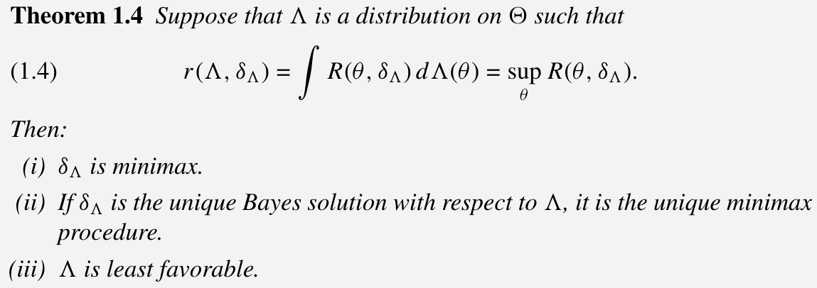
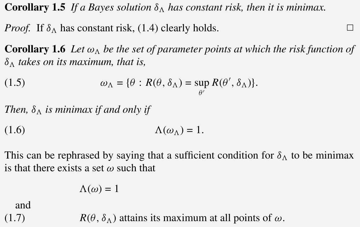
Of two risk functions the one with the smaller maximum is then preferable, and the optimum procedures are those with the minimax property of minimizing the maximum risk.
Since this maximum represents the worst (average) loss that can result from the use of a given procedure, a minimax solution is one that gives the greatest possible protection against large losses.
Maximum Likelihood
the likelihood of $\theta$: the expression $P_\theta(x)$ for fixed $x$ as a function of $\theta$, denoted by $L_x(\theta)$
gain function: $a(\theta)L_x(\theta)$
- maximum-likelihood estimate of $\theta$: assume that $a(\theta)$ is independent of $\theta$, and estimate $\theta$ by the value that maximize the likelihood $L_x(\theta)$.
- likelihood ratio procedure: take decision $d_0$ or $d_1$ as
that is,
\[\frac{\sup_{\theta\in \omega_0}L_x(\theta)}{\sup_{\theta\in\omega_1}L_x(\theta)} > \text{ or }<\frac{a_1}{a_0}\,.\]Complete Classes
Not insisting on a unique solution but asking only how far a decision problem can be reduced without loss of relevant information.
A decision procedure $\delta$ can sometimes be eliminated from consideration because there exists a procedure $\delta’$ dominating it in the sense that
\[\begin{align*} R(\theta,\delta') &\le R(\theta,\delta)\qquad \text{for all }\theta\\ R(\theta,\delta') &< R(\theta,\delta)\qquad \text{for some }\theta\,. \end{align*}\]In this case $\delta$ is said to be inadmissible; $\delta$ is called admissible if no such dominating $\delta’$ exists.
A class $\calC$ of decision procedures is said to be complete if for any $\delta$ not in $\calC$ there exists $\delta’$ in $\calC$ dominating it.
A complete class is minimal if it does not contain a complete subclass. If a minimal complete class exists, it consists exactly of the totality of admissible procedures.
A class $\calC$ is said to be essentially complete if for any procedure $\delta$ there exists $\delta’$ in $\calC$ such that $R(\theta,\delta’)\le R(\theta,\delta)$ for all $\theta$.
Two results concerning the structure of complete classes and minimax procedures have been proved to hold under very general assumptions.
- the totality of Bayes solutions and limits of Bayes solutions constitute a complete class
- minimax procedures are Bayes solutions w.r.t. a least favorable a priori distribution, that is, an a priori distribution that maximizes the associated Bayes risk, and the minimax risk equals this maximum Bayes risk. Somewhat more generally, if there exists no least favorable a priori distribution but only a sequence for which the Bayes risk tends to the maximum, the minimum procedures are limits of the associated sequence of Bayes solutions.
p3111 of TPE
Sufficient Statistics
Reduction of the data: applies simultaneously to all problems relating to a given class $\calP = \{P_\theta,\theta\in \Omega\}$ of distributions of the given random variable $X$.
It consists essentially in discarding that part of the data which contains no information regarding the unknown distribution $P_\theta$, and which is therefore of no value for any decision problem concerning $\theta$.
A statistic $T$ is said to be sufficient for the family $\calP = \{P_\theta:\theta\in \Omega\}$ if the conditional distribution of $X$ given $T=t$ is independent of $\theta$.
A sufficient statistic $T$ is said to be minimal sufficient if the data cannot be reduced beyond $T$ without losing sufficiency.