Subgradient
Posted on
This post is mainly based on Hastie et al. (2015), and incorporated with some materials from Watson (1992).
Consider the convex optimization problem
\[\min_{\beta\in\bbR^p}\;f(\beta)\qquad \text{such that }g_j(\beta)\le 0\text{ for }j=1,\ldots,m\,,\]where $g_j$ are convex functions.
The Lagrangian $L$ is defined as
\[L(\beta;\lambda) = f(\beta) + \sum_{j=1}^m\lambda_jg_j(\beta)\,,\]where the nonnegative weights $\lambda\ge 0$ are known as Lagrange multipliers.
For differentiable problems, the famous KKT (Karush-Kuhn-Tucker) conditions relate the optimal Lagrange multiplier vector $\lambda^*\ge 0$, also known as the dual vector, to the optimal primal vector $\beta^*\in\bbR^p$:
- Primal feasibility: $g_j(\beta^*)\le 0$ for all $j=1,\ldots,m$
- Complementary slackness: $\lambda_j^*g_j(\beta^*)=0$ for all $j=1,\ldots,m$
- Lagrangian conditions: $0=\nabla_\beta L(\beta^*;\lambda^*) = \nabla f(\beta^*)+\sum_{j=1}^m\lambda_j^*\nabla g_j(\beta^*)$.
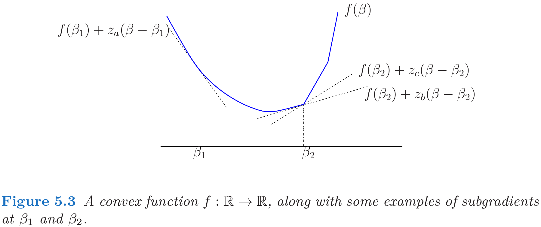
For nondifferentiable functions, there is a natural generalization of the notion of gradient that allows for a more general optimality theory.

Under mild conditions, the generalized KKT theory can still be applied using the modified condition
\[0\in \partial f(\beta^*) + \sum_{j=1}^m \lambda_j^*\partial g_j(\beta^*)\,.\]The remaining parts will give some examples of subgradients.
Subgradients for Lasso
The necessary and sufficient conditions for a solution to
\[\min_{\beta\in\bbR^p} \left\{\frac{1}{2N}\Vert \y-\X\beta\Vert_2^2+\lambda \Vert\beta\Vert_1\right\}\quad \lambda >0\]take the form
\[-\frac 1N\langle \x_j,\y-\X\beta\rangle + \lambda s_j=0,\;j=1,\ldots,p\,.\]Here each $s_j$ is an unknown quantity equal to $\sign(\beta_j)$ if $\beta_j\neq 0$ and some value lying in $[-1,+1]$ otherwise, that is, it is a subgradient for the absolute value function $f(\beta)=\vert \beta\vert$,
\[\partial f(\beta) = \begin{cases} \{+1\} & \text{if }\beta > 0\\ \{-1\} & \text{if }\beta < 0\\ [-1,+1]& \text{if }\beta = 0 \end{cases}\]Subgradients for Nuclear norm
Given a matrix $\Theta\in \bbR^{m\times n}$ (assume $m\le n$), by SVD decomposition,
\[\Theta=\sum_{j=1}^m\sigma_ju_jv_j^T\,.\]The nuclear norm is the sum of the singular values,
\[\Vert \Theta\Vert_*=\sum_{j=1}^m \sigma_j(\Theta)\,.\]The subdifferential $\partial \Vert\Theta\Vert_*$ of the nuclear norm at $\Theta$ consists of all matrices of the form $\Z = \sum_{j=1}^mz_ju_jv_j^T$, where each for $j=1,\ldots,m$, the scalar $z_j\in \sign(\sigma_j(\Theta))$.
Note that we need to verify that
\[\Vert \Theta'\Vert_* \ge \Vert \Theta\Vert_* + \tr[\Z^T(\Theta'-\Theta)]\]for all $\Theta’\in\bbR^{m\times n}$. The inner product for matrix $\A$ and $\B$ is defined by $\langle \A, \B\rangle=\tr(\A^H\B)$
For simplicity, consider the case that all singular values are larger than 0, then
\[\begin{align*} \Vert \Theta\Vert_* + \tr[\Z^T(\Theta'-\Theta)] &= \sum_{j=1}^m \sigma_j + \tr[\V\U^T(\Theta'-\U\D\V^T)] \\ &= \tr[\V\U^T\Theta']\\ &= \tr[\V\U^T\U_*\D_*\V^T_*]\\ &= \sum_{j=1}^m\sigma_j' = \Vert\Theta'\Vert_*\,, \end{align*}\]since $\V\U^T\U_*$ can be viewed as the new left singular vectors.
Subgradient for Orthogonally Invariant Norms
As commented by @Lepidopterist, Watson (1992) completely and thoroughly discussed the derivation of subgradient of (nuclear) matrix norms.
Generally, the subdifferential (or set of subgradients) of $\Vert A\Vert$ is defined by
\[\partial \Vert A\Vert =\left\{G:\bbR^{m\times n}: \Vert B\Vert\ge \Vert A\Vert +\tr[G^T(B-A)], \text{for all }B\in\bbR^{m\times n}\right\}\,.\]It is readily established that $G\in \partial \Vert A\Vert$ is equivalent to the statements
- $\Vert A\Vert = \tr(G^TA)$
- $\Vert G\Vert^*\le 1$
where
\[\Vert G\Vert^* = \max_{\Vert B\vert \le 1}\tr[B^TG]\,,\]and $\Vert \cdot\Vert^*$ is the polar or dual norm to $\Vert \cdot \Vert$.
The class of Orthogonally Invariant Norms consists of norms such that
\[\Vert UVA\Vert =\Vert A\Vert\]for any orthogonal matrices $U$ and $V$ of orders $m$ and $n$ respectively. All such norms can be defined by
\[\Vert A\Vert = \phi(\bsigma)\,,\]where $\bsigma = (\sigma_1,\ldots,\sigma_n)^T$ is the singular values of $A$, and $\phi$ is a symmetric gauge function. For nuclear norm, $\phi(\bsigma_n) = \sum_{j=1}^n\sigma_j$.
I think it does not make much differences for different forms of SVD decomposition.