Wierd Things in Mixture Models
Posted on
This note is based on Larry’s post, Mixture Models: The Twilight Zone of Statistics.
The Gaussian Mixture
One of the simplest mixture models is a finite mixture of Gaussians:
\[p(x,\psi) = \sum_{j=1}^kw_j\phi(x;\mu_j,\Sigma_j)\,.\]Here, $\phi(x;\mu_j,\Sigma_j)$ denotes a Gaussian density with mean vector $\mu_j$ and covariance matrix $\Sigma_j$.
The Wierd Things
Infinite Likelihood
An extreme case pointed by ESL, also by PRML (someone said), the likelihood function can blow up to infinity as the variance of that Gaussian shrinks to zero.
Multimodality of the Likelihood
The likelihood has many modes. Finding the global (but not infinite) mode is a nightmare. The EM algorithm only finds local modes.
Loken (2005) discussed more details about this point.
For a specific application of mixture models, use the following figure which represent the contours of the likelihood to provide some intuition.
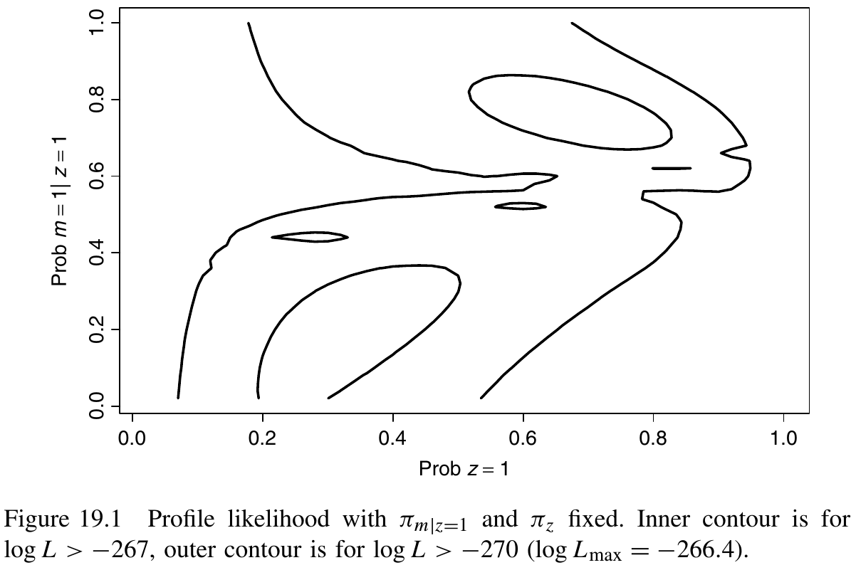
The most notable feature is the two modal regions corresponding to estimates in the neighborhood of the two equivalent maximum likelihood estimates.
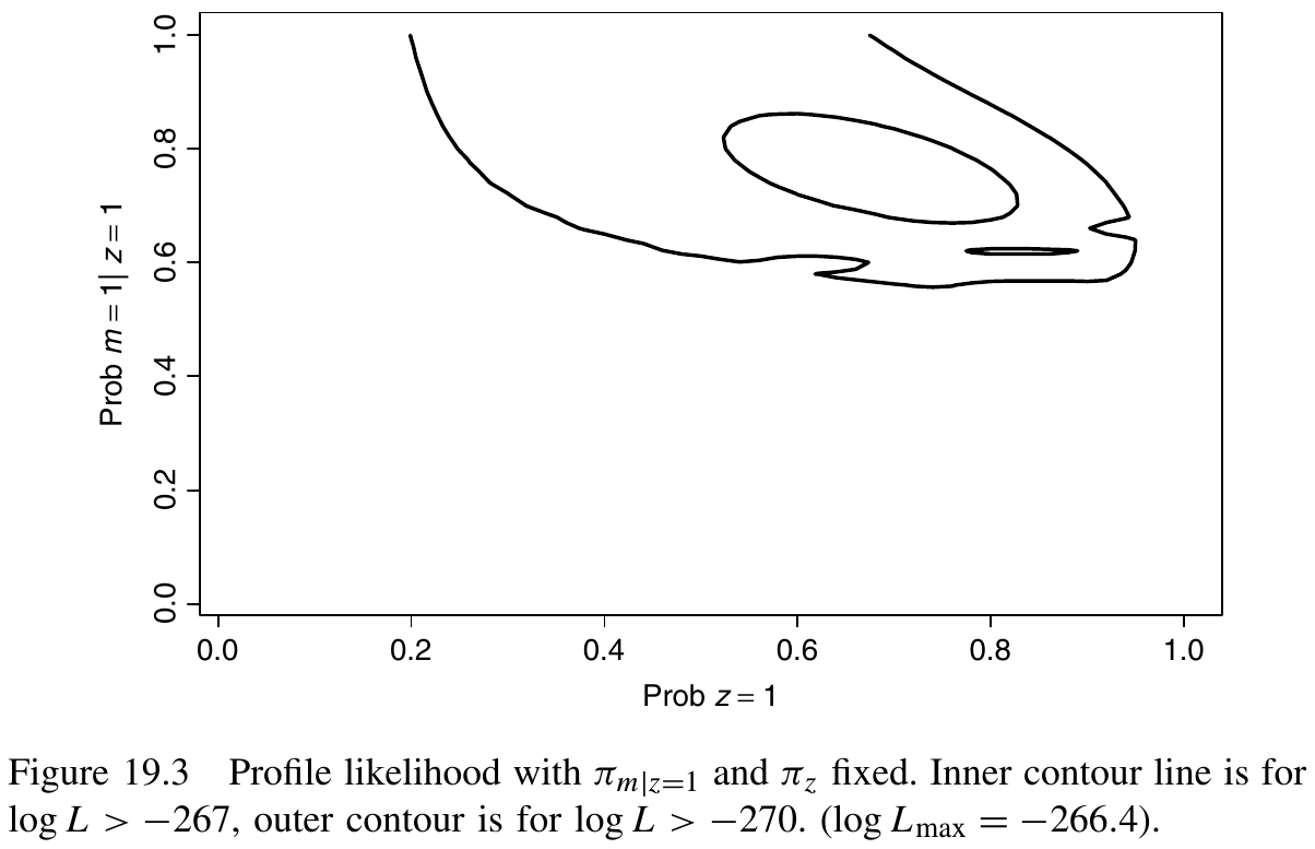
A approach to solve the label-switching problem might be to assign one of the observations to a specific class. If we assume that one of these observations is known to be in class 1, the modified likelihood looks strikingly different.
(I guess there are other modes not caused by the label switching, which would be more serious, but I want some examples to help me understand.)
Multimodality of the Density
The number of modes of a mixture of $k$ Gaussians might have less than $k$ or more than $k$. Edelsbrunner et al. (2013) said that extra (ghost) modes do not exist in $\bbR^1$ and are generally not well studied in high dimensions. They study a configuration of $n+1$ Gaussian kernels for which there are exactly $n+2$ modes.
Nonidentifability
First, there is nonidentifability due to permutation of labels.
Secondly, a bigger issue is local nonidentifability. Suppose that
\[p(x;\eta,\mu_1,\mu_2) = (1-\eta)\phi(x;\mu_1,1) + \eta \phi(x;\mu_2,1)\,.\]- If $\mu_1=\mu_2=\mu$, the parameter $\eta$ has disappeared.
- If $\eta=1$, the parameter $\mu_2$ disappears.
Irregularity
Chen (1995) establish the best possible rate of convergence for estimating the mixing distribution. The key for estimating the mixing distribution is the knowledge of the number of components in the mixture. While a $\sqrt n$-consistent rate is achievable when the exact number of components is known, the best possible rate is only $n^{-1/4}$ when it is unknown.
Nonintuitive Group Membership
Let $Z=1,2$ denote the two components. We can compute $P(Z=1\mid X=x)$ and $P(Z=2\mid X=x)$ explicitly. Then assign an $x$ to the first component if $P(Z=1\mid X=x) > P(Z=2\mid X=x)$.
Improper Posteriors
Improper priors would yield improper posteriors, but proper priors may be undesirable because they require subjective input. Wasserman (2000) proposed the use of specially chose data-dependent priors.
Specifically, let $\cL_n(\psi)$ be the likelihood function and let $\pi(\psi)$ be some ‘target’ prior which assumed to be improper. The formal posterior
\[\pi(\psi\mid Y^n) \propto \cL_n(\psi)\pi(\psi)\]is typically improper. The solution is to replace the likelihood function $\cL_n(\psi)$ with a pseudolikelihood function
\[\cL_n^*(\psi) = \cL_n(\psi) - \inf_\psi\{\cL_n(\psi)\}\,.\]Inference is based on the pseudoposterior
\[\pi^*(\psi\mid Y^n) \propto \cL_n^*(\psi)\pi(\psi)\]which is proper. The pseudoposterior is equivalent to a posterior based on the product of the usual likelihood and a data-dependent prior $\pi_n$, i.e.,
\[\pi^*(\psi\mid Y^n) \propto \cL_n(\psi)\pi_n(\psi)\,.\]References
- Chen, J. (1995). Optimal Rate of Convergence for Finite Mixture Models. The Annals of Statistics, 23(1), 221–233.
- Edelsbrunner, H., Fasy, B. T., & Rote, G. (2013). Add Isotropic Gaussian Kernels at Own Risk: More and More Resilient Modes in Higher Dimensions. Discrete & Computational Geometry, 49(4), 797–822.
- Loken, E. (2005). Multimodality in Mixture Models and Factor Models. In A. Gelman & X.-L. Meng (Eds.), Wiley Series in Probability and Statistics (pp. 203–213).
- Wasserman, L. (2000). Asymptotic Inference for Mixture Models Using Data-Dependent Priors. Journal of the Royal Statistical Society. Series B (Statistical Methodology), 62(1), 159–180.