Tweedie's Formula and Selection Bias

Posted on Mar 11, 2019 (Update: Jan 31, 2020)

Prof. Inchi HU will give a talk on Large Scale Inference for Chi-squared Data tomorrow, which proposes the Tweedie’s formula in the Bayesian hierarchical model for chi-squared data, and he mentioned a thought-provoking paper, Efron, B. (2011). Tweedie’s Formula and Selection Bias. Journal of the American Statistical Association, 106(496), 1602–1614., which is the focus of this note.

Introduction

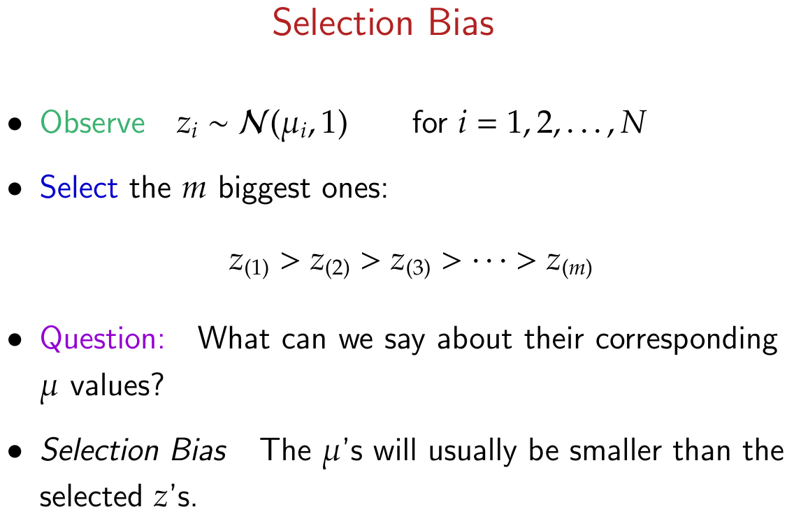
Suppose that some large number $N$ of possibly correlated normal variates $z_i$ have been observed, each with its own unobserved mean parameter $\mu_i$,

where $N=5000$ $\mu_i$ values comprised 10 repetitions each of

and attention focuses on the extremes, say the 100 largest $z_i$’s.

Reproduce Figure 1 with the following Julia code:

using Distributions
using Plots

# figure 1
N = 5000
m = 100
σ = 1
z = ones(N)
μ = repeat(-log.( ( (1:500) .- 0.5) / 500 ), inner = 10)
for i = 1:N
    z[i] = rand(Normal(μ[i], σ))
end
p = histogram(z, legend=false, size = (1080, 720))
for zi in sort(z, rev = true)[1:100]
    plot!(p, [zi, zi], [-5, 0], color = :red)
end
vline!(p, [0])
xlabel!(p, "z values")
ylabel!(p, "Frequency")
savefig(p, "fig1.png")    

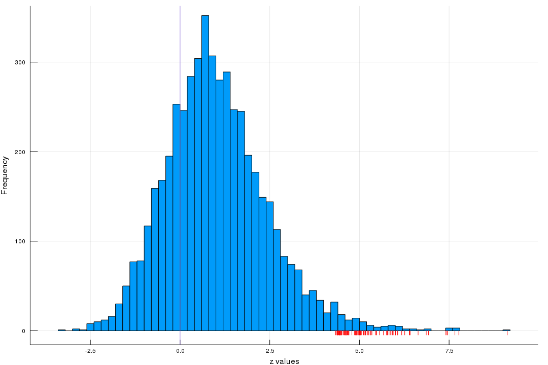
As showed in the following figure in which red dashes on the $y$-axis are the 100 largest $z$’s, while orange stars indicate the corresponding $\mu$ values, it is obvious that $\mu$ is less extreme than $z$.

Here is a great answer to selection bias in Chinese.

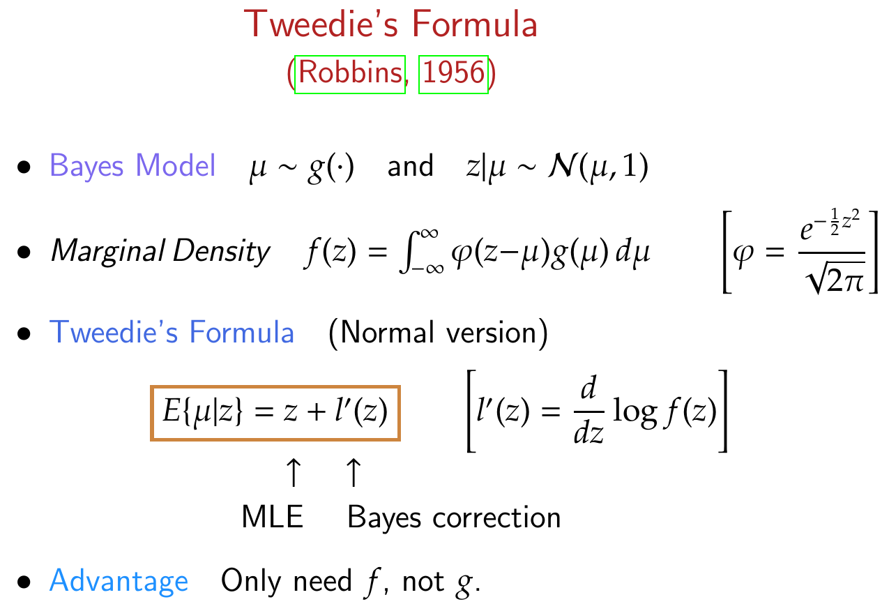
Tweedie’s formula

Consider

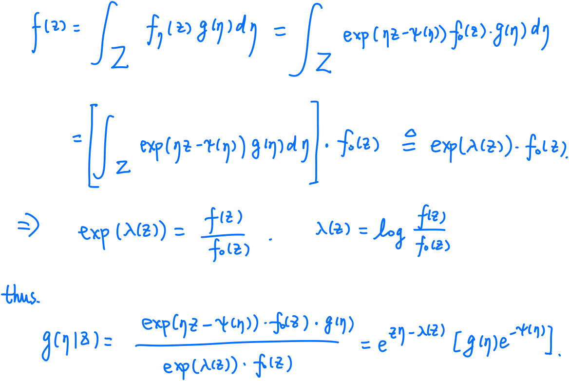
where $\eta$ is the natural or canonical parameter of the exponential family, and $f_0(z)$ is the density when $\eta=0$.

By Bayes rule,

where $f(z)$ is the marginal density

$\cZ$ is the sample space of the exponential family. Then

where $\lambda(z)=\log(f(z)/f_0(z))$.

With the fact of exponential families,

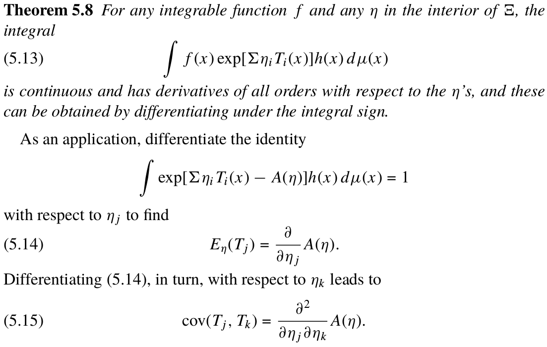
Differentiating $\lambda(z)$ yields

Letting

we can express the posterior mean and variance of $\eta\mid z$ as

In the normal transformation family $z\sim N(\mu,\sigma^2)$, then

and since $\mu=\sigma^2\eta$,

The $N(\mu,\sigma^2)$ family has skewness equal zero. We can incorporate skewness into the application of Tweedie’s formula by taking $f_0(z)$ to be a standardized gamma variable with shape parameter $m$,

in which case $f_0(z)$ has mean 0, variance $1$, and

for all members of the exponential family.

Note that $Z=\frac{Y-m}{\sqrt m}\sim f_0(z)$, then $f_Y(y)=f_0(z)/\sqrt m$, thus

which implies that $\E Y = \frac{m\sqrt m}{\sqrt m-\eta}$, and hence

Since

then

thus we have

There might be a typo in equation (2.13) of Efron (2011)

In summary,

Empirical Bayes Estimation

The empirical Bayes formula

requires a smoothly differentiable estimate of $l(z)=\log f(z)$.

Assume that $l(z)$ is a $J$th-degree polynomial, that is,

which represents a $J$-parameter exponential family having canonical parameter vector $\bbeta=(\beta_1,\ldots,\beta_J)$.

Set the same number of bins $K=63$,

using StatsBase
fit(Histogram, z, nbins= 63)
# Histogram{Int64,1,Tuple{StepRangeLen{Float64,Base.TwicePrecision{Float64},Base.TwicePrecision{Float64}}}}
# edges:
#   -3.4:0.2:9.2
# weights: [1, 0, 2, 1, 8, 10, 12, 16, 30, 50  …  0, 3, 3, 0, 0, 0, 0, 0, 0, 1]
# closed: left
# isdensity: false

the width is also $d=0.2$, with centers $x_k$ ranging from -3.3 to 9.1. The bar heights are given by the weights.

Compare the difference corrected by empirical Bayes, $\hat\mu_i - \mu_i$, and the uncorrected estimate, $z_i-\mu_i$, to check if the empirical Bayes estimate can cure the selection bias.

top100 = sortperm(z, rev=true)[1:100]
∇l(x, f; δ=1e-3) = (f(x .+ δ) - f(x)) / δ
z_density = kde(z)
logf(x) = log.(pdf(z_density, x))
# use derivate of `log f`, NOT `log f`
μhat = z[top100] + ∇l(z[top100], logf)

histogram(μhat - μ[top100], label = "corrected")
histogram!(z[top100] - μ[top100], fillalpha = 0.75, label = "uncorrected")

It is obvious that the empirical Bayes estimate is quite effective since the corrected difference being much more closely centered around zero.

Actually, the simulation is slightly different from Efron (2011), which replicates 100 datasets from the exponential example, and directly simulates $\mu_i$ from $e^{-\mu}$ instead of the approximated $-\log((j-0.5)/500)$.

The empirical Bayes implementation of Tweedie’s formula reduces, almost, to the James-Stein estimator. Suppose the prior density $g(\mu)$ is normal, i.e., $\mu\sim N(0, A)$, and $z\mid\mu\sim N(\mu, 1)$. By the following lemma, the marginal distribution of $z$ is $N(0, V)$, where $V=A+1$,

If $X\mid\theta_1\sim N(\theta_1,\sigma^2_1)$ and $\theta_1\mid\theta_2\sim N(\theta_2,\sigma_2^2)$, where $\sigma_1^2$ and $\sigma_2^2$ are known. Then \(X\mid\theta_2\sim N(\theta_2,\sigma_1^2+\sigma_2^2)\,.\)

Note that

\[\begin{align*} &f(x\mid\theta_2)\\ &= \int f(x\mid \theta_1)\pi(\theta_1\mid\theta_2)d\theta_1\\ &\propto \int \exp\Big(-\frac 12\Big[\big(\frac{x-\theta_1}{\sigma_1}\big)^2+\big(\frac{\theta_1-\theta_2}{\sigma_2}\big)^2\Big]\Big)d\theta_1\\ &=\exp\Big(-\frac 12\Big[\frac{x^2}{\sigma_1^2}+\frac{\theta_2^2}{\sigma_2^2}\Big]\Big)\int\exp\Big(-\frac 12\Big[\frac{1}{\sigma_1^2}+\frac{1}{\sigma_2^2}\Big]\Big[\theta_1-\frac{x/\sigma_1^2+\theta_2/\sigma_2^2}{1/\sigma_1^2+1/\sigma_2^2}\Big]^2+\frac{1}{2}\frac{(x/\sigma_1^2+\theta_2/\sigma_2^2)^2}{1/\sigma_1^2+1/\sigma_2^2}\Big)d\theta_1\\ &\propto \exp\Big(-\frac 12\Big[\frac{x^2}{\sigma_1^2}+\frac{\theta_2^2}{\sigma_2^2}-\frac{(x/\sigma_1^2+\theta_2/\sigma_2^2)^2}{1/\sigma_1^2+1/\sigma_2^2} \Big]\Big)\qquad\text{since the integrand is the pdf of Normal}\\ &=\exp\Big(-\frac{1}{2(\sigma_1^2+\sigma_2^2)}(x-\theta_2)^2\Big)\,, \end{align*}\]

which implies that

\[X\mid\theta_2 \sim N(\theta_2, \sigma_1^2+\sigma_2^2)\,.\]

It follows that $l’(z) = -z/V$ and Tweedie’s formula becomes

where the MLE estimate of $1/V$ is $N/\sum z_j^2$, while the Jame-Stein rule gives

Empirical Bayes Information

The Empirical Bayes Information is the amount of information per “other” observation $z_j$ for estimating $\mu_i$.

For a fixed value $z_0$, let

be the Bayes and empirical Bayes estimates of $\E[\mu\mid z_0]$. Having observed $z=z_0$, the conditional regret for estimating $\mu$ by $\hat\mu_\z(z_0)$ instead of $\mu^+(z_0)$ is

The empirical Bayes information at $z_0$ is defined as

so

Prof. Hu’s Talk

The non-central chi-squared density is a Poisson mixture of central chi-squared densities. Consider the following model

1. Draw the non-centrality parameter $\lambda$ from a prior density $g$.
2. Generate a non-negative integer $J$ according to a Poisson distribution with mean $\lambda/2$
3. Sample from the chi-squared density with $k+2J$ degrees of freedom
4. The resulting $X$ has non-central chi-squared distribution with $k$ DF.

References

• Efron’s slide: Tweedie’s Formula and Selection Bias
• Efron’s slide: Bayes and Empirical Bayes Information