Restricted Boltzmann Machines
Posted on
Boltzmann Machines
Boltzmann Machines are a particular form of log-linear Markov Random Field. In order to make them powerful enough to represent complicated distributions, such as going from the limited parametric setting to a non-parametric one, we introduce the hidden variables (or hidden units). With more hidden units, we can increase the modeling capacity of the Boltzmann Machine.
Consider a graph $G=(V,E)$, which has $p$ visible nodes, termed as $X_j, j=1,2,\ldots, p$, and $X_j$ is a binary variable. Denote the inverse covariance matrix of $X$ as $\mathbf \Theta$, which contains information about the partial covariances between variables. The partial covariances between pairs $i$ and $j$ are the covariances of them conditional on all other variables. In particular, if the $ij$th component of $\mathbf \Theta$ is zero, then variable $i$ and $j$ are conditional independent, given the other variables.
Given some data from this model, the log-likelihood is
\[\begin{align} \ell(\mathbf\Theta)&=\sum\limits_{i=1}^N\mathrm{log\; Pr}_{\mathbf\Theta}(X_i=x_i)\\ &=\sum\limits_{i=1}^N\Big[\sum\limits_{(j,k)\in E}\theta_{jk}x_{ij}x_{ik}-\Phi(\mathbf\Theta) \Big] \end{align}\]The gradient of this log-likelihood is
\[\frac{\partial\ell(\mathbf\Theta)}{\partial\theta_{jk}}=\sum\limits_{i=1}^Nx_{ij}x_{ik}-N\frac{\partial \Phi(\mathbf\Theta)}{\partial\theta_{jk}}\]Now suppose a subset of the variables $X_{\cal H}$ are hidden, and the remainder $X_{\cal V}$ are visible. Then the log-likelihood of the observed data is
\[\begin{align} \ell(\mathbf\Theta)&=\sum\limits_{i=1}^N\mathrm{log}[Pr_{\mathbf\Theta}(X_{\cal V}=x_{i\cal V})]\\ &=\sum\limits_{i=1}^N[\mathrm{log}\sum\limits_{x_{\cal H}\in{\cal X_H}}exp\sum\limits_{(j,k)\in E}(\theta_{jk}x_{ij}x_{jk}-\Phi(\mathbf\Theta))] \end{align}\]The gradient works out to be
\[\frac{d\ell(\mathbf\Theta)}{d\theta_{jk}}=\hat E_{\cal V}E_{\mathbf \Theta}(X_jX_k\mid X_{\cal V})-E_{\mathbf\Theta}(X_jX_k)\]The inner expectation in the first term can be calculated by using basic rules of conditional expectation and properties of Bernoulli random variables. As a result,
\[E_{\mathbf\Theta}(X_jX_k\mid X_{\cal V}=x_{i\cal V}) = \left\{ \begin{array}{ll} x_{ij}x_{ik}& \text{if }j,k\in\cal V\\ x_{ij}Pr_{\cal\mathbf\Theta}(X_k=1\mid X_{\cal V}=x_{i\cal V})&\text{if }j\in\cal V,k\in\cal H\\ Pr_{\mathbf\Theta}(X_j=1,X_k=1\mid X_{\cal V}=x_{i\cal V})&\text{if }j,k\in{\cal H} \end{array} \right.\]In principle, we can implement two separate runs of Gibbs sampling.
- Estimate $E_{\mathbf\Theta}(X_jX_k)$ by sampling from the model.
- Estimate $E_{\mathbf\Theta}(X_jX_k\mid X_{\cal V}=x_{i\cal V})$
However, this procedure can be very slow. Fortunately, restricted Boltzmann machines can make these computations manageable.
Restricted Boltzmann Machines

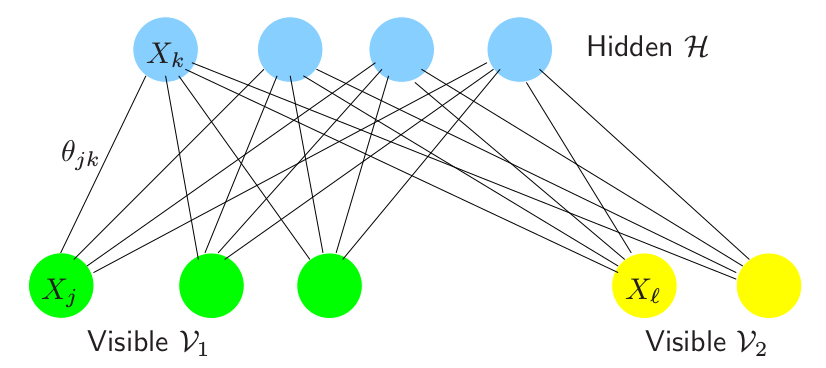
As you can see in the above figure, a restricted Boltzmann Machine is a Boltzmann machine in which there are no connections between nodes in the same layer. Then the conditional expectation can be easier,
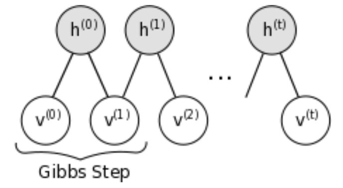
\[E_{\Theta}(X_jX_k\mid X_{\cal V}=x_{i\cal V})= \left\{ \begin{array}{ll} x_{ij}x_{ik}&\text{if }j,k\in\cal V\\ Pr_{\Theta}(X_j=1,X_k=1\mid X_{\cal V}=x_{i\cal V})&\text{if }j,k\in\cal H \end{array} \right.\]Considering the fact that the set of visible and hidden units are conditionally independent. So we can sample visible units simultaneously given fixed values of the hidden units. Similarly, hidden units can be sampled simultaneously given the visible units. A schematic diagram is as follows.

Implement on MNIST
There is a python program which use restricted Boltzmann machine to recognize hand-written digits from the MNIST dataset. In this program, it constructs a RBM with 784 visible units and 500 hidden units, using contrastive divergence. But it did not use the label information. You can find the code in the first reference at the end of this post.