Growing A Polymer
Posted on (Update: )
This report implements the simulation of growing a polymer under the self-avoid walk model, and summary the sequential importance sampling techniques for this problem.
Model: Self-avoid walk
For the sake of a concise description of the model, we just consider two-dimensional lattice space.
In such a model, the realization of a chain polymer of length $N$ is fully characterized by the positions of all of its molecules, $\mathbf x = (x_1, x_2,\ldots, x_N)$, where $x_i = (a, b)$ is a point in the 2-D lattice space. The distance between $x_i$ and $x_{i+1}$ has to be exactly 1, and $x_{i+1}\neq x_k, k<i$
A possible Boltzmann distribution for the chain polymer modeled by an SAW is the uniform distribution. More formally, the target distribution of interest in this case is \(\pi(\mathbf x)=\frac{1}{Z_N}\) where the space of $\mathbf x$ is the set of all SAWs of length $N$ and $Z_N$ is the normalizing constant, which is just the total number of different SAWs with $N$ atoms.
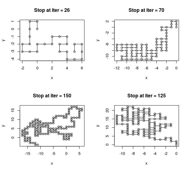
Let $x_1 = (0, 0), x_2=(1, 0)$. Draw the position of $x_{t+1}$ conditional on the current configuration of $(x_1, \ldots, x_t)$, according to the probability distribution
\[P(x_{t+1} = (i', j')\mid x_1,\ldots, x_t) = \frac{1}{n_t}\]where $(i’, j’)$ is one of the unoccupied neighbors of $x_t$ and $n_t$ is the total number of such unoccupied neighbors.
Unfortunately, the SAWs produced by this way is not uniformly distributed. Considering the target distribution is $\pi(\mathbf x)\propto 1$ and the sampling distribution of $\mathbf x$ is $(n_1\times \cdots\times n_{N-1})^{-1}$, so assign a weigh
\[w(\mathbf x) = n_1\times \cdots\times n_{N-1}\]to the SAW.
Implement this simple model by using the following R code
Sequential importance sampling
Apply the sequential importance sampling, there are two alternatives for auxiliary sequence of distribution.
Firstly, consider the sequence of auxiliary distributions $\pi_t(\mathbf x_t), t=1,\ldots, N-1$ is just the sequence of auxiliary distributions of SAWs with $t$ nodes, where $Z_t$ is the total number of such SAWs. Under $\pi_t$, the marginal distribution of the partial sample $\mathbf x_{t-1}=(x_1,\ldots, x_{t-1})$ is
\[\pi_t(x_{t-1})= \sum\limits_{x_t}\pi_t(\mathbf x_{t-1}, x_t) = \frac{n_{t-1}}{Z_t}\]Then, $\pi_t(x_t\mid \mathbf x_{t-1})=1/n_{t-1}$, so we can choose the sampling distribution $g_t(x_t\mid \mathbf x_{t-1})$ as $1/n_{t-1}$. If $n_{t-1} = 0$, $g(x_t\mid \mathbf x_{t-1}) = 0.$
In addition to this auxiliary distributions, we can use the marginal distribution of $\mathbf x_t$ under the uniform distribution of $(\mathbf x_t, x_{t+1})$
\[\pi_t'(\mathbf x_t)=\sum\limits_{x_{t+1}}\frac{1}{Z_{t+1}}\propto n_t\]then we can let $g_t$ be $\pi_t’(x_t\mid \mathbf x_{t-1})$. This procedure is equivalent to a two-step-look-ahead approach.
We can compute certain descriptive statistics regarding such SAWs, say the mean squared extension of the chain $E\Vert x_N-x_1\Vert^2$ or the total number of possible configuration of SAWs with $N$ nodes $Z_N$.
In order to estimate $Z_N$, consider the importance weight. We can compute the importance weight recursively as \(\begin{aligned} w_{t+1} & = \frac{\pi_{t+1}(\x_{1:t+1})}{g_{t+1}(\x_{1:t+1})}\\ &= \frac{\pi_{t}(\x_{1:t})}{g_t(\x_{1:t})}\frac{\pi_{t+1}(\x_{1:t+1})}{\pi_{t}(\x_{1:t})g_{t+1}(x_{t+1}\mid \x_{1:t})}\\ &=w_tn_t\,. \end{aligned}\)
Then we obtain
\[w_N = \prod\limits_{t=1}^{N-1}n_t \cdot w_1 = \prod\limits_{t=2}^N\frac{1}{g_t(x_t\mid x_1,\ldots, x_{t-1})}\]The target distribution is $\pi(\mathbf x) = \frac{1}{Z_N}$, the weight satisfies the relationship \(w_N = Z_N\pi(\mathbf x)/p(\mathbf x)\)
Hence, $E_p(w_N) = Z_N$, which gives us a means to estimate the partition function (normalizing constant):
\[\hat Z_N = \bar w_N\]where $\bar w_N$ is the sample average of the weights obtained by repeating the biased sampling procedure multiple, say $m$, times.
References
Liu, Jun S. Monte Carlo strategies in scientific computing. Springer Science & Business Media, 2008.