Model Specification
Posted on
For a given time series, how to choose appropriate values for $p, d, q$
Sample Autocorrelation Function
For the observed time series, $Y_1,\ldots, Y_n$, we have
\[r_k = \frac{\sum\limits_{t=k+1}^n(Y_t-\bar Y)(Y_{t-k}-\bar Y)}{\sum\limits_{t=1}^n(Y_t-\bar Y)^2},\; for\; k=1,2,\ldots\]For $MA(q)$ models, the ACF is zero for lags beyond $q$, so the sample autocorrelation is a good indicator of the order of the process.
The Partial Autocorrelation Functions
To help to determine the order of autoregressive models, a function may be defined as the correlation between $Y_t$ and $Y_{t-k}$ after removing the effect of the intervening variables $Y_{t-1}, Y_{t-2},\ldots, Y_{t-k+1}$. This coefficient is called the partial autocorrelation at lag $k$.
There are several ways to make the definition precise.
If $\{Y_t\}$ is a normally distributed time series, let
\[\phi_{kk} = Corr(Y_t, Y_{t-k}\mid Y_{t-1}, Y_{t-2},\ldots, Y_{t-k+1})\]An alternative approach, NOT based on normality, can be developed in the following way. Consider predicting $Y_t$ based on a linear function of the intervening variables $Y_{t-1}, Y_{t-2},\ldots, Y_{t-k+1}$, say, $\beta_1Y_{t-1} + \ldots + \beta_{k-1}Y_{t-k+1}$, with the $\beta$’s chosen to minimize the mean square error of prediction. Then assuming $\beta$ have been chosen and then think backward in time, it follows from stationary that the best “predictor” of $Y_{t-k}$ based on the same $Y_{t-1},Y_{t-2},\ldots, Y_{t-k+1}$ will be $\beta_1Y_{t-k+1}+\ldots+\beta_{k-1}Y_{t-1}$. (??) The partial autocorrelation function at lag $k$ is then defined to be the correlation between the prediction error,
\[\phi_{kk} = Corr(Y_t-\beta_1Y_{t-1}-\beta_2Y_{t-2}-\cdots-\beta_{k-1}Y_{t-k+1}, Y_{t-k}-\beta_1Y_{t-k+1}-\beta_2Y_{t-k+2}-\cdots -\beta_{k-1}Y_{t-1})\]For an AR(p) model,
\[\phi_{kk} = 0\; for\; k>p\]The sample partial autocorrelation function (PACF) can be estimated recursively.
The Extended Autocorrelation Functions
The EACF method uses the fact that if the AR part of a mixed ARMA model is known, “filtering out” the autoregressive from the observed time series results in a pure MA process that enjoys the cutoff property in its ACF.
As the AR and MA orders are unknown, an iterative procedure is required. Let
\[W_{t,k,j} = Y_t-\tilde \phi_1 Y_{t-1} -\cdots - \tilde \phi_kY_{t-k}\]be the autoregressive residuals defined with the AR coefficient estimated iteratively assuming the AR order is $k$ and the MA model is $j$. The sample autocorrelations of $W_{t,k,j}$ are referred to as the extended sample autocorrelation.
Nonstationarity
To avoid overdifferencing, we recommend looking carefully at each difference in succession and keeping the principle of parsimony always in mind—models should be simple, but not too simple
The Dickey-Fuller Unit-Root Test.
AIC or BIC
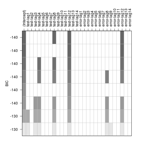
Order determination is related to the problem of finding the subsets of nonzero coefficients of an ARMA model with sufficiently high ARMA orders. A subset $ARMA(p, q)$ model is an $ARMA(p,q)$ model with a subset of its coefficients known to be zero. For example, the model
\[Y_t = 0.8Y_{t-12}+e_t+0.7e_{t-12}\]is a subset ARMA(12, 12) model useful for modeling some monthly seasonal time series.
