The Gibbs Sampler

Posted on Jun 04, 2017 (Update: Mar 12, 2019) 0 Comments

Gibbs sampler is an iterative algorithm that constructs a dependent sequence of parameter values whose distribution converges to the target joint posterior distribution.

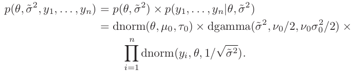
A semiconjugate prior distribution

In the case where $\tau_0^2$ is not proportional to $\sigma^2$, the marginal density of $1/\sigma^2$ is not a gamma distribution.

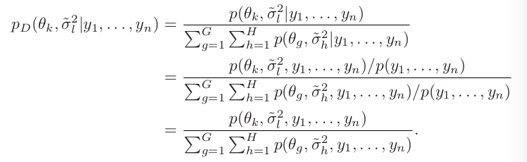
Discrete approximations

A discrete approximation to the posterior distribution makes use of these facts by constructing a posterior distribution over a grid of parameter values, based on relative posterior probabilities.

Construct a two-dimensional grid of value of ${\theta, \tilde \sigma^2}$

An example

mu0 = 1.9; t20 = 0.95^2; s20 = 0.01; nu0 = 1
y = c(1.64, 1.70, 1.72, 1.74, 1.82, 1.82, 1.82, 1.90, 2.08)
G = 100; H = 100
mean.grid = seq(1.505, 2.00, length = G)
prec.grid = seq(1.75,175, length = H)
post.grid = matrix(nrow = G, ncol = H)

for (g in 1:G){
    for (h in 1:H){
        post.grid[g, h] =
            dnorm(mean.grid[g], mu0, sqrt(t20)) *
            dgamma(prec.grid[h], nu0/2, s20*nu20/2) *
            prod(dnorm(y, mean.grid[g], 1/sqrt(prec.grid[h])))
    }
}
post.grid = post.grid/sum(post.grid)

Sampling from the conditional distributions

if we know $\theta$, we can easily sample directly from $p(\sigma^2\mid \theta,y_1,\ldots,y_n)$. And we can easily sample from $p(\theta\mid\sigma^2,y_1,\ldots,y_n)$.

1. suppose we sample from the marginal posterior distribution $p(\sigma^2\mid y_1,\ldots, y_n)$ and obtain $\sigma^{2(1)}$.

2. then we could sample $\theta^{(1)}\sim p(\theta\mid \sigma^{2(1)},y_1,\ldots,y_n)$, and {$\theta^{(1)},\sigma^{2(1)}$} would be a sample from the joint distribution of {$\theta,\sigma^2$}.

3. $\theta^{(1)}$ could be considered a sample from the marginal distribution $p(\theta\mid y_1,\ldots,y_n)$. For this $\theta$-value, sample $\sigma^{(2)}\sim p(\sigma^2\mid \theta^{(1)},y_1,\ldots,y_n)$

4. {$\theta^{(1)},\sigma^{2(2)}$} is also a sample from the joint distribution of {$\theta,\sigma^2$}. This in turn means that $\sigma^{2(2)}$ is a sample from the marginal distribution $p(\sigma^2\mid y_1,\ldots,y_n)$, which then could be used to generate a new sample $\theta^{(2)}$.

Gibbs sampling

the full conditional distributions \(p(\theta\mid \sigma^2,y_1,\ldots,y_n)\) and \(p(\sigma^2\mid \theta,y_1,\ldots,y_n)\)

given a current state of the parameters \(\phi^{(s)}=\{\theta^{(s)}, \tilde \sigma^{2(s)}\}\)

generate a new state as follows

1. sample $\theta^{(s+1)}\sim p(\theta\mid \tilde\sigma^{2(s)},y_1,\ldots,y_n)$
2. sample $\tilde\sigma^{2(s+1)}\sim p(\tilde\sigma^2\mid \theta^{(s+1)},y_1,\ldots,y_n)$
3. let $\phi^{(s+1)}={\theta^{s+1},\tilde\sigma^{2(s+1)}}$

General properties of the Gibbs sampler

Markov property, Markov chain.

the sampling distribution of $\phi^{(s)}$ approaches the target distribution as $s \rightarrow \infty $, no matter what the starting value $\phi^{(0)}$ is (although some starting values will get you to the target sooner than others).

More importantly, for most functions $g$ of interest,

the necessary ingredients of a Bayesian data analysis are

1. Model specification: $p(y\mid \phi)$
2. Prior specification: $p(\phi)$
3. Posterior summary: $p(\phi\mid y)$

Remarks:

Monte Carlo and MCMC sampling algorithms

• are not models
• do not generate “more information” than is in $y$ and $p(\phi)$
• simply “ways of looking at” $p(\phi\mid y)$

for example,

Distinguishing parameter estimation from posterior approximation

Introduction to MCMC diagnostics

difference between MC and MCMC

1. Independent MC samples automatically create a sequence that is representative of $p(\phi)$: The probability that $\phi\in A$ for any set $A$ is $\int_A p(\phi) d\phi$. This is true for every $s \in {1, . . . , S}$ and conditionally or unconditionally on the other values in the sequence.
2. NOT true for MCMC, instead we have

Two types of Gibbs sampler

Suppose we can decompose the random variable into $d$ components, $\mathbf x=(x_1,\ldots, x_d)$. In the Gibbs sampler, one randomly or symmetrically chooses a coordinate, say $x_1$, then updates it with new sample $x_1’$ draw from the conditional distribution $\pi(\cdot\mid \mathbf x_{[-1]})$.

Random-scan Gibbs Sampler

Let $\mathbf x^{(t)}=(x_1^{(t)},\ldots, x_d^{(t)})$ for iteration $t$. Then, at iteration $t+1$, conduct the following steps:

• Randomly select a coordinate $i$ from ${1, \ldots, d}$ according to a given probability vector $(\alpha_1, \ldots, \alpha_d)$
• Draw $x_{i}^{(t+1)}$ from the conditional distribution $\pi(\cdot\mid x_{[-i]}^{(t)})$ and leave the remaining components unchanged

Systematic-Scan Gibbs Sampler

Let $\mathbf x^{(t)}=(x_1^{(t)},\ldots, x_d^{(t)})$ for iteration $t$. Then, at iteration $t+1$,

• Draw $x_i^{i+1}$ from the conditional distribution

In the both samplers, at every update step, $\pi$ is still invariant. Suppose $\mathbf x^{(t)}\sim \pi$, then $\mathbf x_{[-i]}^{(t)}$ follows its marginal distribution under $\pi$. Thus,

which means that after one conditional update, the new configuration still follows distribution $\pi$.

References

• Hoff, P. D. (2009). A first course in Bayesian statistical methods. London; New York: Springer.
• Liu, Jun S. Monte Carlo strategies in scientific computing. Springer Science & Business Media, 2008.