Illustrations of Support Vector Machines
Posted on
Use the e1071 library in R to demonstrate the support vector classifier and the SVM.
Implement in R
library(e1071)
svm() ## kernel = "linear"
## small "cost" means wide margins, while large "cost" means narrow margins
An intuition is that large “cost” $C$ would be more strict for the misclassification, and hence narrow margins. Specially, $C = \infty$ corresponds to the separable case.
Refer to 12.2 支持向量分类器 - ESL CN for more details.
Support Vector Classifier
demonstration for two-dimensional example
generate the data
set.seed(1)
x = matrix(rnorm(20*2), ncol = 2)
y = c(rep(-1 ,10), rep(1 ,10) )
x[y == 1, ] = x[y == 1, ] + 1
plot(x , col = 3-y )
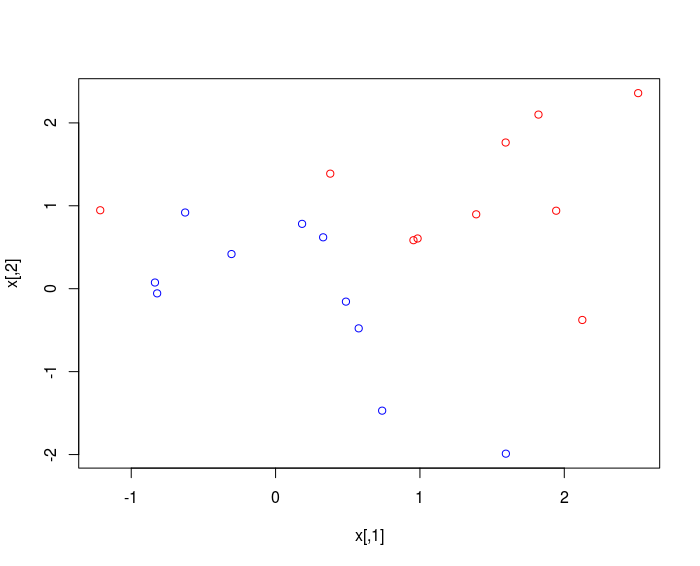
The classes are NOT linearly separable.
fit the support vector classification
It is worth noting that we must encode the response as a factor variable in order to perform classification.
dat = data.frame(x = x, y = as.factor(y))
library(e1071)
svmfit = svm (y ~ ., data = dat, kernel = "linear", cost = 10, scale = FALSE)
plot(svmfit, dat)
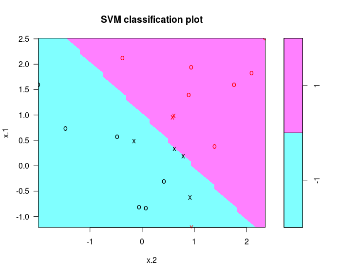
determine the identities
svmfit$index
summary(svmfit)
a smaller cost
svmfit = svm ( y ∼. , data = dat, kernel = "linear" , cost = 0.1, scale = FALSE )
plot(svmfit, dat)
svmfit$index
After setting a smaller cost, we will get a larger number of support vectors, because the margin is now wider.
cross-validation
We can use ``tune()” to perform ten-fold cross-validation on a set of models of interest.
set.seed(1)
tune.out = tune (svm, y ~ ., data = dat, kernel ="linear",
     ranges = list ( cost = c (0.001 , 0.01 , 0.1 , 1 ,5 ,10 ,100) ) )
The output is as follows:
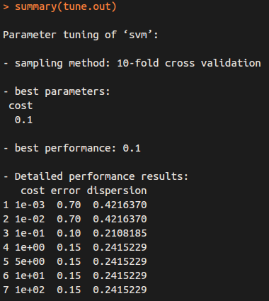
So “cost = 0.1” results in the lowest cross-validation error rate, and we can access the best model as follows:
bestmod = tune.out$best.model
summary( bestmod )
prediction
xtest = matrix ( rnorm (20*2) , ncol =2)
ytest = sample ( c ( -1 ,1) , 20 , rep = TRUE )
xtest [ ytest ==1 ,]= xtest [ ytest ==1, ] + 1
testdat = data.frame ( x = xtest , y = as.factor ( ytest ) )
ypred = predict ( bestmod , testdat )
table ( predict = ypred , truth = testdat$y )
Support Vector Machine
generate some data with a non-linear class boundary
set.seed(1)
x = matrix ( rnorm (200*2) , ncol =2)
x [1:100, ]= x [1:100, ]+2
x [101:150, ]= x [101:150, ] -2
y = c ( rep(1, 150) , rep(2, 50) )
dat = data.frame ( x =x , y = as.factor ( y ) )
plot(x, col = y)
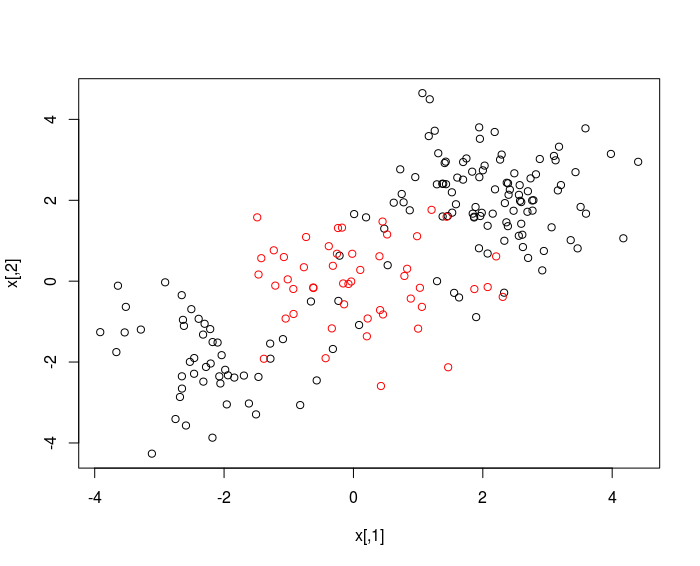
randomly split into training and testing groups.
train = sample (200 ,100)
training data using radical kernel
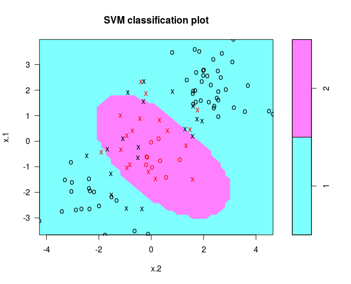
svmfit = svm(y~. , data = dat [ train ,], kernel = "radial", cost =1)
plot ( svmfit , dat [ train ,])
cross-validation
set.seed (1)
tune.out = tune(svm, y∼. , data = dat [ train ,] , kernel =" radial " ,
     ranges = list ( cost = c (0.1 ,1 ,10 ,100 ,1000) ,
     gamma = c (0.5 ,1 ,2 ,3 ,4) ) )
summary( tune.out )
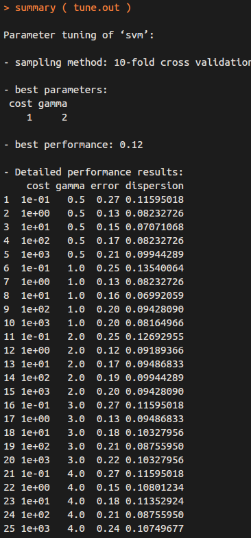
Therefore, the best choice of parameters involves “cost=1” and “gamma=2”.
prediction
table( true = dat [ - train ,"y"] , pred = predict ( tune.out$best.model, newdata = dat [ - train ,]) )
ROC Curves
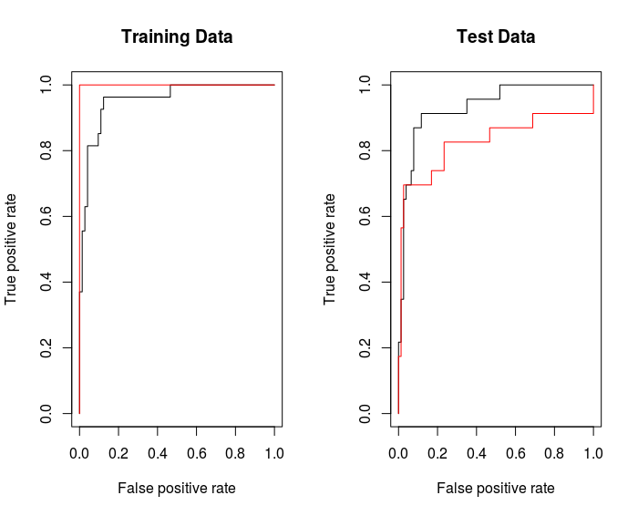
The ROC curve is a popular graphic for simultaneously displaying the two types of errors for all possible thresholds.
Varying the classifier threshold changes its true positive rate (sensitivity) and false positive rate (1 - specificity).


The overall performance of a classifier, summarized over all possible thresholds, is given by the area under the (ROC) curve (AUC). An ideal ROC curve will hug the top left corner, so the larger the AUC the better the classifier.
The ROCR package can be used to produce ROC curves.
library(ROCR)
rocplot = function ( pred , truth , ...) {
         predob = prediction ( pred, truth )
         perf = performance ( predob , "tpr" , "fpr")
         plot ( perf,...) }
svmfit.opt = svm (y~., data = dat[train, ], kernel = "radial", gamma =2 , cost =1 , decision.values = T )
fitted = attributes(predict(svmfit.opt, dat[train, ], decision.values = TRUE))$decision.values
par ( mfrow = c (1 ,2) )
rocplot ( fitted , dat [ train ,"y"] , main ="Training Data")
By increasing $\gamma$ we can produce a more flexible fit and generate further improvements in accuracy.
svmfit.flex = svm(y~. , data = dat [ train ,] , kernel = "radial", gamma =50 , cost =1 , decision.values = T )
fitted = attributes ( predict ( svmfit.flex , dat [ train ,] , decision.values = T ) ) $decision.values
rocplot ( fitted , dat [ train ,"y"] , add =T , col ="red")
But on the test data, $\gamma = 2$ would be better.
fitted = attributes(predict(svmfit.opt, dat[-train, ], decision.values = T ) ) $decision.values
rocplot(fitted, dat[-train, "y"] , main = "Test Data")
fitted = attributes(predict(svmfit.flex, dat[-train, ], decision.values = T ) ) $decision.values
rocplot(fitted, dat[-train, "y"] , add =T, col ="red")
SVM with Multiple Classes
set.seed (1)
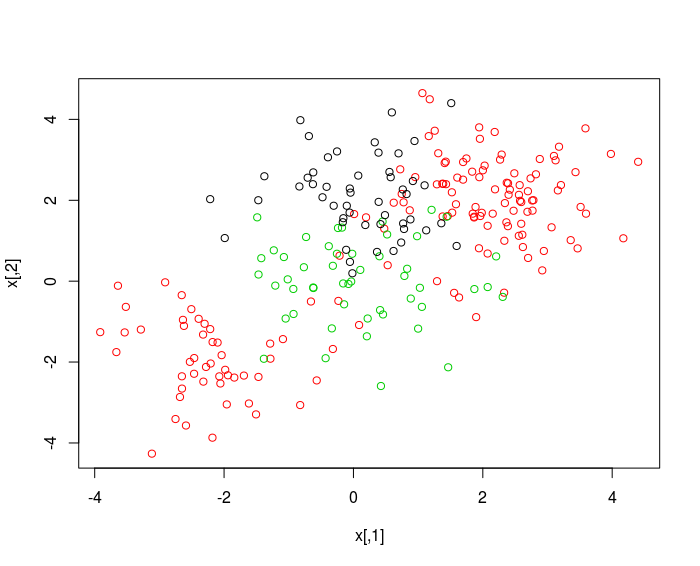
x = rbind (x, matrix ( rnorm (50*2) , ncol =2) )
y = c ( y , rep (0 ,50) )
x [ y ==0 ,2]= x [ y ==0 ,2]+2
dat = data.frame ( x =x , y = as.factor ( y ) )
par(mfrow = c (1 ,1) )
plot (x , col = (y +1) )
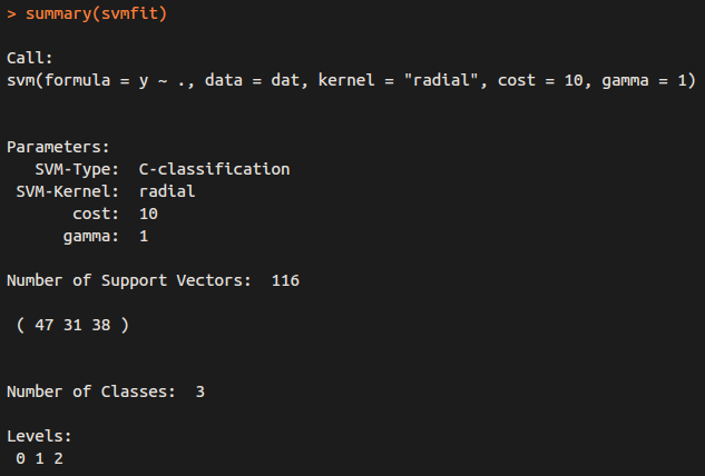
svmfit = svm(y~., data = dat , kernel ="radial" , cost =10 , gamma =1)
plot ( svmfit , dat )
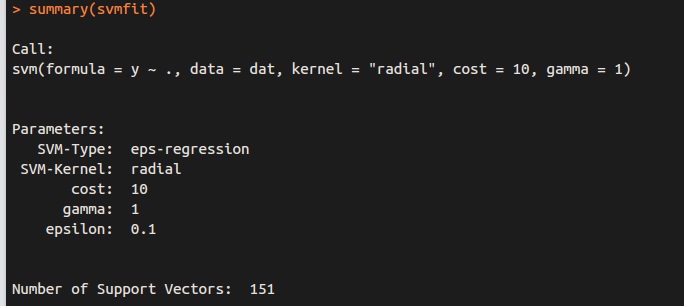
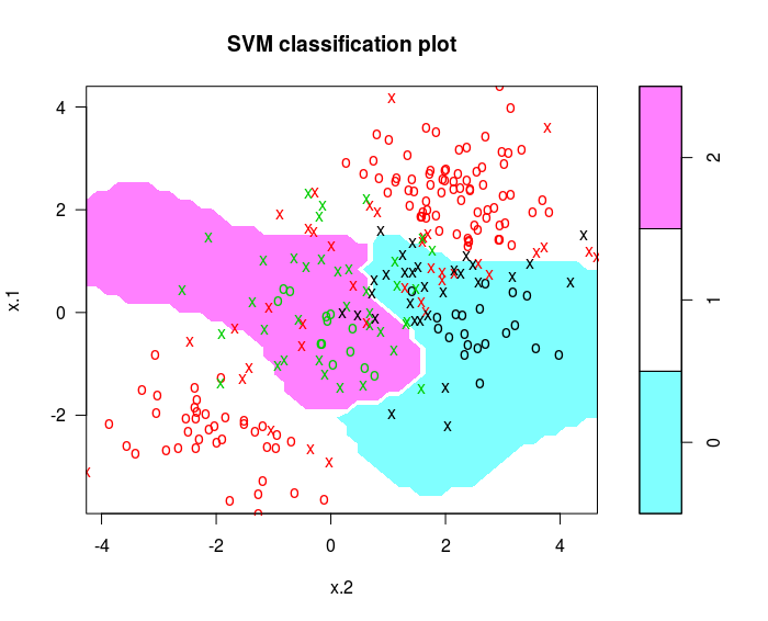 The e1071 library can also be used to perform support vector regression, if the response vector that is passed in to svm() is numerical rather than a factor.
for classification (y is factor)
for regression (y is NOT factor)
Application to Gene Expression Data
examine the dimension of the data
library(ISLR)
names(Khan)
dim(Khan$xtrain)
dim(Khan$xtest)
length(Khan$ytrain)
length(Khan$ytest)
table(Khan$ytrain)
table(Khan$ytest)
dat = data.frame ( x = Khan$xtrain, y = as.factor(Khan$ytrain))
out = svm ( y~., data = dat , kernel = "linear", cost =10)
summary(out)
table ( out$fitted , dat$y )
NO training errors. In fact, this is not surprising, because the large number of variables relative to the number of observations implies that it is easy to find hyperplanes that fully separate the classes.
dat.te = data.frame ( x = Khan$xtest , y = as.factor( Khan$ytest ) )
pred.te = predict ( out, newdata = dat.te )
table ( pred.te , dat.te$y )
Reference
An Introduction to Statistical Learning with Applications in R