Variable Importance Measure for Heterogeneous Treatment Effect
Posted on
VIM for heterogeneous treatment effects
- introduce nonparameteric treatment effect variable importance measures (TE-VIMs), based on the MSE in predicting the individual treatment effect.
- TE-VIMs represent the increase in MSE when variables are removed from the CATE conditioning set.
CATE:
\[\tau(x) = E(Y^1 - Y^0\mid X=x)\]- one pioneering proposal for CATE variable attribution: extend random forest variable importance measures (VIMs) through the causal forest estimator of the CATE
- VIMs based on specific modeling strategies (decision tree, linear regression, etc.) are referred to as “algorithmic”
- While algorithmic-VIMs can provide useful insights, there remains a need for model-agnostic alternatives, especially when the chosen CATE estimating strategy does not have a well-established algorithmic-VIM
- propose treatment effect variable importance measures (TE-VIMs) that are nonparameteric summary statistics, which measure the importance of variable subsets in predicting the individual treatment effect (ITE) $Y^1 - Y^0$
consider the mean-sqaured-error
\[L(f) = E[(Y^1-Y^0-f(X))^2]\]one key insight
\[L(f) = E[(\tau(X) - f(X))^2] + E[\var(Y^1-Y^0\mid X)]\]define the TE-VIM
\[\Theta_s = L(\tau_s) - L(\tau)\]where
\[\tau_s(x) = E(Y^1-Y^0\mid X_{-s} = x_{-s})\]is the CATE conditional on $X_{-s}$
We have \(\Theta_s = E[(\tau(X) - \tau_s(X))^2]\,.\)
Since \(\tau_s(X) = E[\tau(X)\mid X_{-s}]\)
Thus \(\Theta_s = E[\Var(\tau(X)\mid X_{-s})]\)
Then by total variance decomposition, \(\Var(\tau(X)) = \Var(\tau_s(X)) + E[\Var(\tau(X)\mid X_{-s})]\)
which implies \(\Theta_s = \Var(\tau(X)) - \Var(\tau_s(X))\)
the variance $\var(\tau(X))$ of the treatment effect (VTE), a global measure of treatment effect heterogeneity
- $\Theta_s$: quantifies the treatment effect heterogeneity explained by $X_s$ beyond that already explained by $X_{-s}$
TE-VIMs connects to regression-VIMs, also called “leave-out covariates”
2 Methodology
2.1 Motivating the estimand
- $\tau_p$: the average treatment effect (ATE)
- $\Theta_p$: VTE
personally speaking, i felt we can write $\tau_{[p]}$ to avoid misleading
assuming
- consistency: $A=a \Rightarrow Y=Y^a$
- conditional exchangeability: $Y^a\ind A\mid X$ for $a=0, 1$
- positivity: $0 < \pi(x) < 1$ almost surely
the CATE is identified by
\[\tau(x) = \mu(1, x) - \mu(0, x)\]where
\[\mu(a, x) = E(Y\mid A=a, X=x)\]and $\pi(x) = E(A\mid X=x)$ is the propensity score.
Assuming $\Vert \tau(X)\Vert <\infty$, then the TE-VIM
\[\Theta_s = \Vert \tau(X) - \tau_s(X)\Vert^2 < \infty\]is also finite.
the TE-VIM $\Theta_s$ is analogous to the regression-VIM
\[\Omega_s = \Vert Y-\mu_s(X)\Vert^2 - \Vert Y-\mu(X)\Vert^2\]propose scaled TE-VIMs as
\[\Psi_s = \Theta_s / \Theta_p = 1-\Var(\tau_s(X)) / \Theta_p\]modes:
- leave-one-out
- keep-one-in
- shapley values
- covariate grouping
2.2 CATE estimation
- metalearning strategies decompose CATE estimation into a sequence of subregression problems, which can be solved using off-the-shelf ML algorithms
- 2 metalearning algorithms: T-learner and DR-learner
- T-learner is based on the decomposition \(\tau(x) = \mu(1, x) - \mu(0, x)\) and estimate the CATE by \(\hat\tau^{(T)}(x) = \hat\mu(1, x) - \hat\mu(0, x)\)
- the T-learner is problematic for 2 main reasons:
- while regularization methods can be used to control the smoothness of $\hat\mu(a, x)$, the same is not true of $\hat\tau^{(T)}(x)$ which may be erratic. Slow convergence rate affecting $\hat\mu(a, x)$ may therefore propagate into $\hat\tau^{(T)}(x)$.
- $\hat\mu(1, x)$ is chosen to make an optimal bias-variance trade-off over the covariance distribution of the treated population. Likewise, $\hat\mu(0, x)$ is chosen to make an optimal bias-variance trade-off over the covariate distribution of the untreated population. When there is poor overlap between the treated and untreated subgroups, then $\hat\tau^{(T)}(x)$ may fail to deliver an optimal bias-variance trade-off over the population covariate distribution, making the T-learner potentially poorly targeted toward CATE estimation.
- the DR-learner is an alternative metalearning algorithm based on the decomposition \(\tau(x) = E[\phi(Z)\mid X=x]\) where, for $z = (y, a, x)$
is called the pseudo outcome, or the augmented inverse propensity weighted (AIPW) score, and acts like the ITE in expectation.
- the DR-learner first estimates $\mu(a, x)$ and $\pi(x)$ to obtain the pseudo-outcome estiator $\hat\phi(Z)$, where $\mu(a, x)$ and $\pi(x)$ are replaced with estimates $\hat\mu(a, x)$ and $\hat\pi(x)$
- in a second step, the estimated pseudo-outcome, $\hat\phi(Z)$ is regressed on covariates $X$ to obtain $\hat\tau^{(DR)}(x)$.
- The DR-learner alleviates the issues related to the T-learner since the complexity of $\hat\tau^{(DR)}(x)$ can be controlled by regularizing the regression in the final stage of the procedure.
- one can trade-off accuracy in the outcome and propensity score estimators, a property known as double robustness, hence the name “DR-learner”
- estimation of the CATE $\tau_s(x)$ is complicated by the fact that one cannot assume that $Y\ind A\mid X_{-s}$ for an arbitrary subset of covariates $s$, a problem that is sometimes referred to as “runtime confounding”
- the DR-learner readily accommodates runtime confounding through the identity $\tau_s(x) = E[\phi(Z)\mid X_{-s}=x_{-s}]$. The identity implies that one may estimate $\tau_s(x)$ by regressing $\hat\phi(Z)$ on $X_{-s}$, that is, modifying the final regression step of the DR-learner.
2.3 TE-VIM estimation
2.3.1 Estimation of $\Theta_s$
consider estimators based on the efficient influence curve (IC) of $\Theta_s$ under the nonparameteric model.
ICs are mean 0 functions that characterize the sensitivity of so-called pathwise differentiable estimands to small changes in the data generating law.
ICs are useful for constructing efficient estimators and determining their asymptotic distribution
since the risk $L[f]$ is not identified. Consider that
\[\Theta_s = L_U[\tau_s] - L_U[\tau]\]where
\[L_U[f]= E[(U+\tau(X) - f(X))^2] = E[(\tau(X) - f(X))^2] + E[U^2]\]and $U$ is a random variable such that $E[U\mid X] = 0$. Note that $U = Y^1 - Y^0 - \tau(X)$ recovers the unidentified risk $L(f)$ and $U = \phi(Z)-\tau(X)$ recovers the DR-learner population risk
consider the risk $L^\star(f)$ obtained by setting $U=0$.
the IC of $L^\star(f)$ at a single observation $z$ is
\[[\phi(z) - f(x)]^2 - [\phi(z) - \tau(x)]^2 -L^\star[f]\]the IC of $\Theta_s$ is
\[\phi_s(z) = [\phi(z) - \tau(x)]^2 - [\phi(z) - \tau(x)]^2 - \Theta_s\]\[\Theta_s = E[\tau(X)^2] - E[\tau_s(X)^2]\,.\]The AIPW pseudo-outcome is
\(\varphi(Z) = \tau(X) + \frac{A}{e(X)}(Y-m_1(X)) - \frac{1-A}{1-e(X)}(Y-m_0(X))\) It satisfies \(E[\varphi(Z)\mid X] = \tau(X)\) Write \(\varepsilon(Z) = \varphi(Z) - \tau(X)\) Then \(E[\varepsilon(Z)\mid X] = 0\) The role of $\varphi - \tau$ is important: it is the influence-function contribution for perturbations of the conditional outcome distributions that determine $\tau(X)$
EIF of $\Psi_1 = E[\tau(X)^2]$
note that for any mean parameter $E(W)$, the influence function is \(W - E(W)\)
Suppose temporarily that $\tau(X)$ were directly observed and fixed. Then the influence function arising from changes in the marginal distribution of $X$ would simply be \(\tau(X)^2 -\Psi_1\,.\)
But $\tau(X)$ is itself an unknown conditional mean. Differentiating the square gives the multiplier. The influence-function contribution from estimating $\tau(X)$ is therefore \(2\tau(X)[\varphi(Z) - \tau(X)]\)
Combining the two parts gives \(\phi_1(Z) = 2\tau(X)[\varphi(Z) - \tau(X)] + \tau(X)^2 - \Psi_1\)
Similar for EIF of $\Psi_2$
EIF of $\Psi_2 = E[\tau_s(X)^2]$
\[\phi_2(Z) = 2\tau_s(X)\varphi(Z) -\tau_s(X)^2 -\Psi_2\,.\]Thus, \(\phi_s(Z) = 2(\tau-\tau_s)\varphi -\tau^2 +\tau_s^2 - \Phi_s\)
it can be written as \(\phi_s(Z) = (\varphi(Z) - \tau_s(X))^2 - (\varphi(Z) - \tau(X))^2 - \Phi_s\)
the interpretation of $\phi(Z)$ as a pseudo-outcome, which plays the role of the unobserved ITE $Y^1 - Y^0$
2.3.2 Importance testing
$H_0: \Theta_s = 0$
in which case $\phi_s(Z) = 0$. This IC degeneracy makes $H_0$ difficult to test, since $\hat\Theta_s$ is not necessarily asymptotically normal.
one solution to the IC degeneracy problem is to estimate $\var(\tau(X))$ and $\var(\tau_s(X))$ using efficient estimators in separate samples
2.3.3 Estimation of $\Psi_s$
the scaled TE-VIM
\[\Psi_s = \Theta_s / \Theta_p\]hac IC
\[\Phi_s(z) = (\phi_s(z) - \Psi_s\phi_p(z)) / \Theta_p\]General chain rule
Suppose $\Psi = g(\eta_1, \eta_2)$, where $\eta_1$ has EIF $\phi_1$, and $\eta_2$ has EIF $\phi_2$
Then \(\phi_\Psi = \frac{\partial g}{\partial \eta_1}\phi_1 + \frac{\partial g}{\partial \eta_2}\phi_2\)
The estimator $\hat\Theta_p$ and $\hat\Psi_s$ both rely on an ATE estimator $\hat\tau_p$.
The IC of the ATE, $\phi(z) - \tau_p$, implies an efficient estimator
\[\hat\tau_p^\star = n^{-1}\sum_{i=1}^n \hat\phi(z_i)\]known as the AIPW estimator
2.3.4 Plug-in estimation
a common framework for constructing debiased estimators is through targeted maximum likelihood estimators (TMLEs)
2.3.5 Algorithms
3 Simulation Study
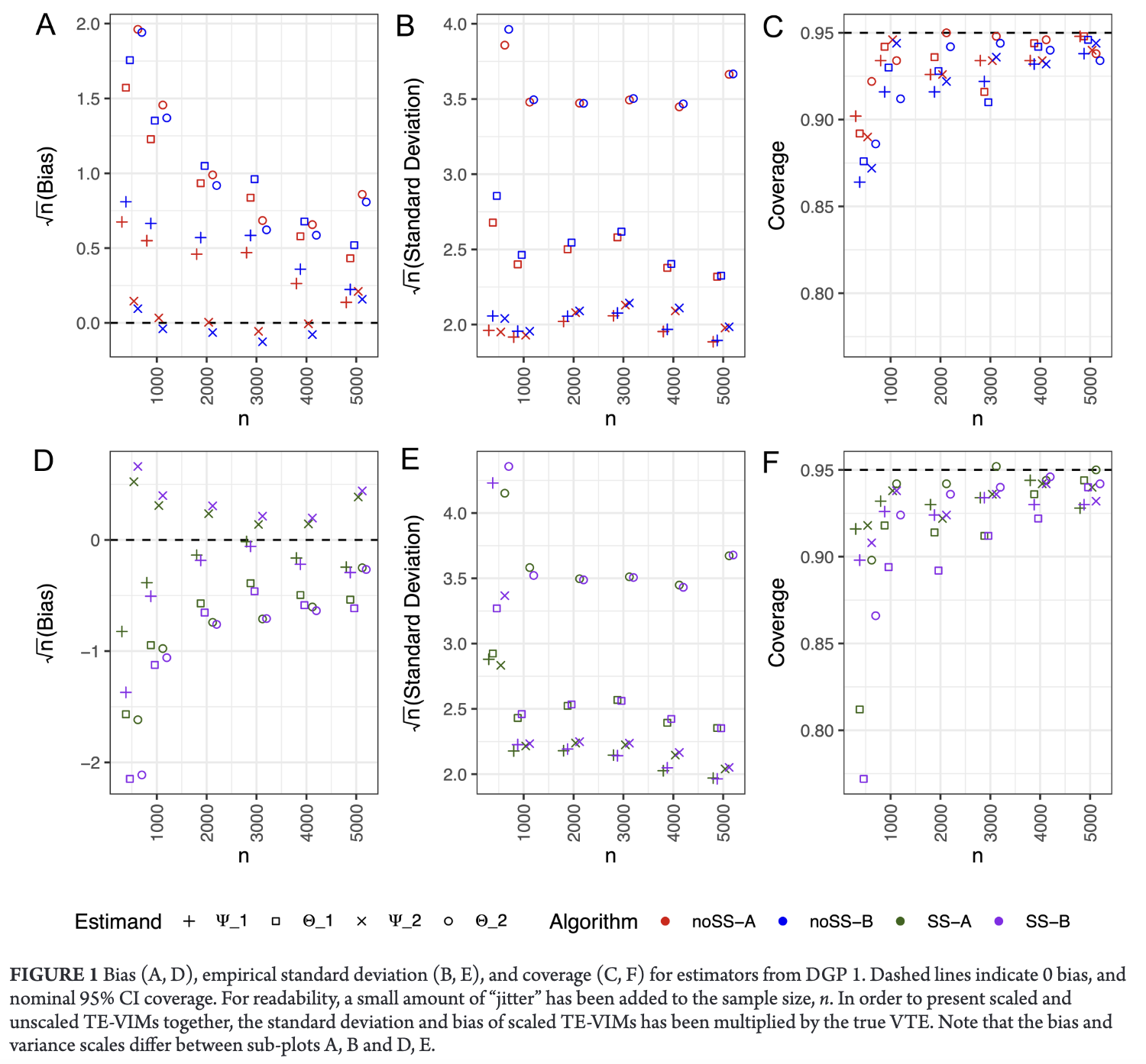
DGP 1
\[X_1, X_2 \sim U(-1, 1), \quad A\sim \text{Bernoulli}(-0.4X_1+0.1X_1X_2)\] \[\tau^{(1)}(X) = X_1^3 + 1.4X_1^2 + 25X_2^2/9\]and
\[Y \sim N_1(X_1X_2 + 2X_2^2 - X_1 + A\tau^{(1)}(X), 1)\]Thus, \(EX_1^2 = EX_2^2 = 1/3\) and hence
  # consider cate of the form: a X1^2 + b X2^2 + c X1^3
  ate <- (a + b) / 3
and \(\Var(aX_1^2 + bX_2^2 + cX_1^3) = E[(aX_1^2+bX_2^2+cX_1^3)^2] - [E(aX_1^2 + bX_2^2 + cX_1^3)^2]\) where \(E[(aX_1^2+bX_2^2+cX_1^3)^2] = E[a^2X_1^4 + b^2X_2^4 + c^2X_1^6 + 2abX_1^2X_2^2 + 2acX_1^5 + 2bcX_1^3X_2^2]\\ = E[a^2X_1^4 + b^2X_2^4 + c^2X_1^6 + 2abX_1^2X_2^2]\\ = a^2/5 + b^2/5 + c^2/7 + 2ab / 9\) thus
    te_sq <- c^2 / 7 + (a^2 + b^2) / 5 + 2 * a * b / 9
    vte <- te_sq - ate^2
thus
vte = c^2/7 + (a^2+b^2) (1/5 - 1/9)Hence
tevim_1 = vte - Var(tau_1) = c^2 / 7 + a^2 * (1/5 - 1/9)
tevim_2 = vte - Var(tau_2) = b^2 * (1/5 - 1/9)
tevim_1_scaled = tevim_1 / vte
tevim_2_scaled = tevim_2 / vte
The calculated results are: ```r true_vals_dgp1 <- true_values(1.4, 25 / 9, 1) true_vals_dgp1 $ate [1] 1.392593
$vte [1] 1.00295
$tevim_1 [1] 0.3170794
$tevim_1_scaled [1] 0.3161466
$tevim_2 [1] 0.6858711
$tevim_2_scaled [1] 0.6838534 ```
{.comment}
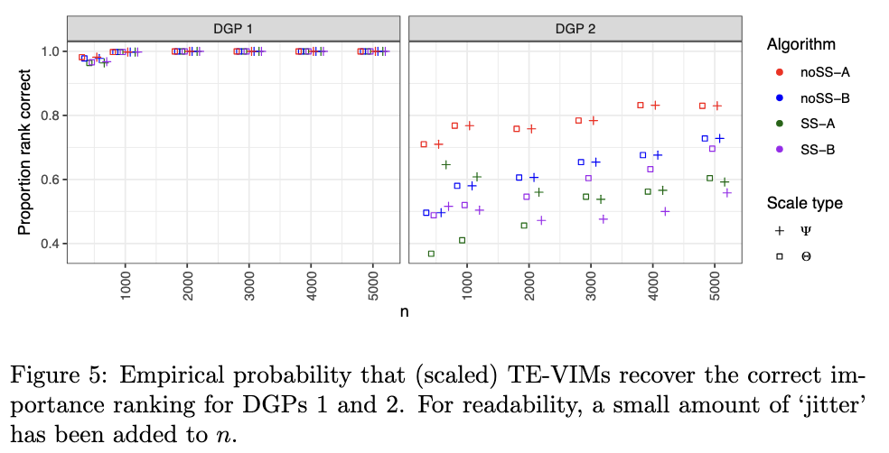
report the empirical probability that TE-VIMs correctly rank $X_2$ as more important than $X_1$
DGP 3
\[(X_1, X_2), (X_3, X_4), (X_5, X_6) \sim N(0, \begin{pmatrix} 1 & 0.5\\ 0.5 & 1 \end{pmatrix})\] \[A\sim \text{Bernoulli}(\text{expit}(-0.4X_1 + 0.1X_1X_2 + 0.2X_5))\] \[\tau^{(3)}(X) = X_1 + 2X_2 + X_3\] \[Y\sim N(X_3-X_6+A\tau^{(3)}(X), 3)\]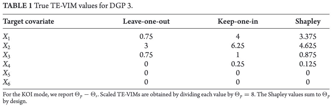
4 Applied Example: AIDS Clinical Trial
2139 HIV patients with CD4 T-cell count between 200 and 500 mm$^{-3}$ randomized to 4 treatment groups
- compare groups (ii) and (iii) (A = 0, 1), with 561 and 522 patients
- consider CD4 count at 20 ± 5 weeks as a continuous outcome Y and 12 baseline covariates, 5 continuous: age, weight, Karnofsky score, CD4/CD8 count; and 7 binary: sex, homosexual activity (y/n), race (white/non-white), symptomatic (y/n), intravenous drug use history(y/n), hemophilia (y/n), and antiretroviral history (experienced/naive).