A modern maximum-likelihood theory for high-dimensional logistic regression

Posted on Jul 18, 2026

Tags: Logistic Regression

This is the note for Sur, Pragya, and Emmanuel J. Candès. “A Modern Maximum-Likelihood Theory for High-Dimensional Logistic Regression.” Proceedings of the National Academy of Sciences 116, no. 29 (2019): 14516–25.

consider a logistic model with independent features in which $n$ and $p$ become increasingly large in a fixed ratio. The paper proves that

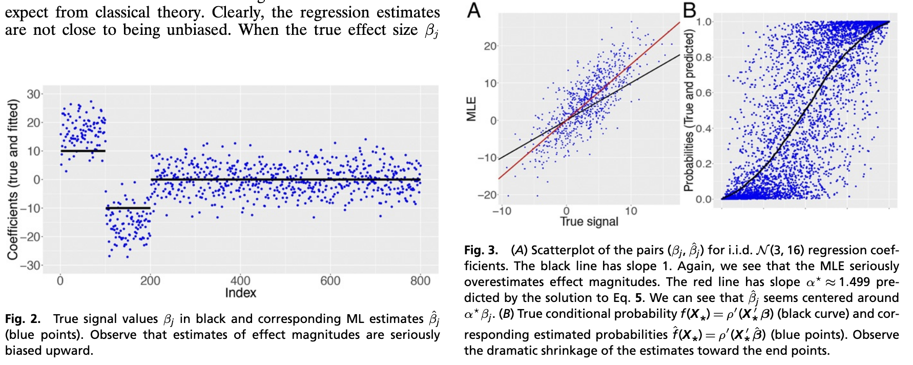
• the maximum-likelihood estimate is biased
• the variability of the MLE is far greater than classically estimated
• the likelihood-ratio test (LRT) is not distributed as a $\chi^2$

2 Contribution

a useful feature of this theory is that in the model, all of the results depend on the true coefficients $\beta$ only through the signal strength $\gamma$, where $\gamma^2 = \Var(X_i’\beta)$

3 Prior Work

4 Main Results

$p/n\rightarrow\kappa> 0$

assume $X_i\sim N(0, n^{-1}I_p)$

the exact scaling of $X_i$ is not important. The important scaling is the signal strength $X_i’\beta$ and we assume that the $p$ regression coefficients are scaled in such a way that

\[\lim_{n\rightarrow\infty} \Var(X_i'\beta) = \gamma^2\]

where $\gamma$ is fixed.

4.a When Does the MLE Exist?

The MLE $\hat\beta$ is the minimizer of the negative log-likelihood $\ell$ defined via

\[\ell(b) = \sum_{i=1}^n\{\rho(X_i'b) - y_i(X_i'b)\}, \quad \rho(t) = \log(1+e^t)\]

a first important remark is that in high dimensions, the MLE does not asymptotically exist if the signal strength $\gamma$ exceeds a certain functional $g_{MLE}(\kappa)$ of the dimensionality

4.b A system of nonlinear equations

the asymptotic behavior of both the MLE and the LRT is characterized by a system of equations in three variables $(\alpha, \sigma,\lambda)$

4.c The average behavior of the MLE

\[\frac 1p\sum_{j=1}^p \psi(\hat\beta_j - \alpha_\star\beta_j, \beta_j) \overset{a.s.}{\rightarrow} \bbE[\psi(\sigma_\star Z, \beta)], Z\sim N(0, 1)\]

4.d The distribution of the null MLE coordinates

\[\hat\beta_j\overset{d}{\rightarrow} N(0, \sigma^2_\star)\]

4.e The Distribution of the LRT

\[2\Lambda_j \overset{d}{\rightarrow} \frac{\kappa \sigma_\star^2}{\lambda_\star}\chi_1^2\]

the LLR is stochastically much larger than a $\chi_1^2$

4.f other scalings

4.g Non-Gaussian Covariates

5. Adjusting Inference by Estimating the Signal Strength

5.a ProbeFrontier: Estimating $\gamma$ by Probing the MLE Frontier

Given a data sample $(y_i, X_i)$, we begin by choosing a fine grid of values $\kappa\le \kappa_1\le\kappa_2 \ldots \le \kappa_K\le 1/2$.

For each $\kappa_j$, execute the following procedure:

1. subsample: sample $n_j = p/\kappa_j$ observations from the data without replacement. The dimensionality if this subsample is $p/n_j = \kappa_j$
2. check whether MLE exists: for the subsample, check whether the MLE exists or not. This is done by solving a linear programming feasibility problem;
   • if there exists a vector $b\in \IR^p$ such that $X_i’b$ is positive when $y_i = 1$ and negative otherwise, then perfect separation between cases and controls occurs and the MLE does not exist.
   • if the linear program is infeasible, then the MLE exists.
3. repeat. repeat the two previous steps $B$ times and compute the proportion of times $\hat \pi(\kappa_j)$ the MLE does not exist.

next find $(\kappa_{j-1}, \kappa_j)$, such that $\kappa_j$ is the smallest value for which $\hat\pi(\kappa_j) \ge 0.5$.

By linear interpolation between $\kappa_{j-1}$ and $\kappa_j$, obtain $\hat\kappa$ for which the proportion of times the MLE does not exist would be 0.5.

5.b Empirical Performance of Adjusted Inference

5.c Debiasing the MLE and Its Predictions

6 Broader Implications and Future Directions

• correlated predictors
• robustness of p values to model misspecifications