Similarity Network Fusion
Posted on (Update: )
This post is for Wang, B., Mezlini, A. M., Demir, F., Fiume, M., Tu, Z., Brudno, M., Haibe-Kains, B., & Goldenberg, A. (2014). Similarity network fusion for aggregating data types on a genomic scale. Nature Methods, 11(3), Article 3. and a related paper Ruan, P., Wang, Y., Shen, R., & Wang, S. (2019). Using association signal annotations to boost similarity network fusion. Bioinformatics, 35(19), 3718–3726.
- $n$ samples, such as patients, ${x_1,\ldots,x_n}$
- $m$ measurements, such as
- patient similarity network $G = (V, E)$
- similarity matrix $W$
- $\rho(x_i, x_j)$: Euclidean distance between patients $x_i$ and $x_j$
where
- $\mu$: a hyperparameter that can be empirically set, and recommend it in the range of $[0.3, 0.8]$ why?
- $\varepsilon_{i,j}$ is used to eliminate the scaling problem
- normalized weight matrix $P=D^{-1}W$, where $D$ is the diagonal matrix with $D(i, i) = \sum_j W(i, j)$ so that $\sum_{j}P(i, j)=1$, but this normalization may suffer from numerical instability since it involves self-similarities on the diagonal entries of $W$.
- one way to perform a better normalization, which is free of the scale of self-similarity in the diagonal entries and $\sum_j P(i, j)=1$ still holds.
- let $N_i$ represent a set of $x_i$’s neighbors including $x_i$ in $G$. Given a graph, $G$, use $K$ nearest neighbors (KNN) to measure local affinity as
two data types
when we have two data types, $m=2$,
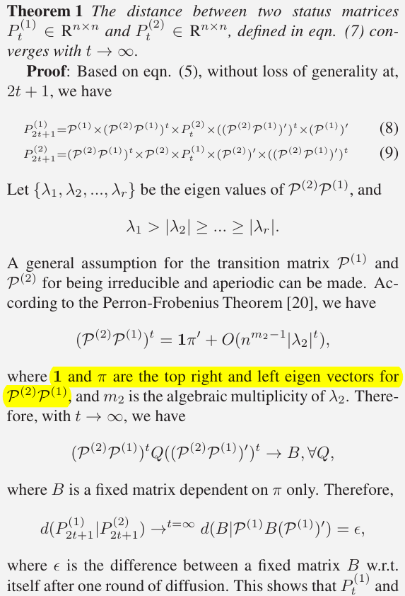
- let $P_{t=0}^{(1)}=P^{(1)}, P_{t=0}^{(2)}=P^{(2)}$ represent the initial two status matrices at $t=0$.
the key step of SNF is to iteratively update similarity matrix corresponding to each of the data types
\[\begin{align*} P_{t+1}^{(1)} &= S^{(1)} \times P_t^{(2)} \times (S^{(1)})^T\\ P_{t+1}^{(2)} &= S^{(2)} \times P_t^{(1)} \times (S^{(2)})^T \end{align*}\]After $t$ steps, the overall status matrix is computed as
\[P^{(c)} = \frac{P_t^{(1)}+ P_t^{(2)}}{2}\]Another way to think of the updating rule is
\[P_{t+1}^{(1)}(i, j) = \sum_{k\in N_i}\sum_{l\in N_j} S^{(1)}(i, k)\times S^{(1)}(j, l)\times P_t^{(2)}(k, l)\]which implies that the similarity information is only propagated through the common neighborhood. This renders SNF robust to noise.
after each iteration, performed normalization on $P_{t+1}^{(1)}$ and $P_{(t+1)}^{(2)}$, which ensured that
- throughout SNF iterations a patient is always most similar to himself than to other patients
- our final network is full rank, important for the classification and clustering applications of the final network
and the paper claims that the use of such normalization leads to quicker convergence of SNF
screenshot at the same first author’s work on computer vision Wang, B., Jiang, J., Wang, W., Zhou, Z.-H., & Tu, Z. (2012). Unsupervised metric fusion by cross diffusion. 2012 IEEE Conference on Computer Vision and Pattern Recognition, 2997–3004.
Let $A$ be an $n\times n$ positive matrix. Then
- There is a positive real number $r$, called the Perron root or the Perron-Frobenius eigenvalue, such that $r$ is an eigenvalue of $A$ and any other eigenvalue $\lambda$ (possibly complex) in absolute value is strictly smaller than $r$.
- There exists an eigenvector $v$ of $A$ with eigenvalue $r$ such that all components of $v$ are positive: $Av=rv, v_i > 0$. Respectively, there exists a positive left eigenvector $w$: $w^TA=rw^T, w_i > 0$.
- $\lim_{k\rightarrow\infty} A^k/r^k = vw^T$, where the left and right eigenvectors for $A$ are normalized so that $w^Tv=1$.
source: wikipedia
an extension to the case $m > 2$ is
\[P^{(\nu)} = S^{(\nu)}\times \left(\frac{\sum_{k\neq \nu}P^{(k)}}{m-1}\right)\times (S^{(\nu)})^T\,,\nu = 1,2,\ldots,m\]Network Clustering
associate each sample $x_i$ with a label indicator vector $y_i\in{0, 1}^C$ such that $y_i(k)=1$ if sample $x_i$ belongs to the $k$-th cluster (subtype), otherwise $y_i(k)=0$.
So a partition matrix $Y=(y_1^T,y_2^T,\ldots,y_n^T)$ is used to represent a clustering scheme.
Traditional state-of-the-art spectral clustering method, aim to minimize RatioCut, an objective function that effectively combines MinCut and equipartitioning, by solving the following optimization problem
\[\min_{Q\in \IR^{n\times C}} \text{Trace}(Q^TL^+Q) \quad \text{s.t.} Q^TQ=I\,,\]where $Q = Y(Y^TY)^{-1/2}$ is a scaled partition matrix, $L^+$ denotes the normalized Laplacian matrix $L^+=I - D^{-1/2}WD^{-1/2}$ and $D$ is a network degree matrix, with degrees of each node on the diagonal and off-diagonal elements set to 0.
Network-based survival risk prediction
Given all the feature matrix $X$, the risk of an event (death) at time $t$ for the $i$-th patient something wrong is given by
\[h(t\mid X) = h_0(t)\exp(X^Tz)\,,\]where $z$ is a vector of regression coefficients and $h_0(t)$ is the baseline hazard function.
The regression coefficient vector $z$ is estimated by maximizing the Cox’s log-partial likelihood
\[\text{lp}(z) = \sum_{i=1}^n \delta_i\left(X_i^Tz - \log \left(\sum_{j\in R(t_i)}\exp(X_j^Tz)\right) \right)\]where
- $t_i$ is the survival time for the $i$-th patient
- $R(t_i)$ is the risk set at time $t_i$, i.e., the set of patients who still survived before $t_i$
- $\delta_i(\cdot)$ is an indicator function whether the survival time is observed $\delta_i=1$ or censored $\delta_i=0$.
To incorporate the network structure, similarity between either features or patients (or both) can be used as a regularizer. According to the hazard function of Cox’s model, the relative risk between patient $i$ and patient $j$ is $\exp(X_i^Tz-X_j^Tz)$, therefore, a regularizer can be constructed as $(X_i^Tz-X_j^Tz)^2w_{ij}$. To estimate $z$, we can use a modified likelihood expression as follows
\[lp(z) = \sum_{i=1}^n\delta_i\left(X_i^Tz - \log \left(\sum_{j\in R(t_i)}\exp(X_j^Tz)\right) \right)-\lambda\sum_i\sum_j(X_i^Tz-X_j^Tz)^2w_{ij}\,,\]where $\lambda$ is the regularizing coefficient.
Compatibility of data sources can be checked via normalized mutual information (NMI). If the patient similarity obtained from different data sources is completely discordant; NMI can help to clarify which data should be and which should not be combined.
Ruan et al. (2019)’s weighted distance in SNF
The paper proposed an association-signal-annotation boosted similarity network fusion (ab-SNF) method: adding feature-level association signal annotations as weights aiming to up-weight signal features and down-weight noise features when constructing subject similarity networks to boost the performance in disease subtyping.
For individual types of omics data, consider features that can better differentiate tumor samples from adjacent normal samples (or independent normal samples) as potential signal features for subtyping tumor samples, i.e., features with stronger association signals with outcome of interests. The authors want to up-weight these signal features in constructing the patient similarity network using this type of omics data.
- for a continuous feature $k$ such as an epigenetic feature (DNA methylation at a CpG site) or a transcriptomic feature (gene expression of a gene), weight the feature using the feature-level association p-value $p_k$ from comparing tumor samples to adjacent normal samples (or independent normal samples) at feature $k$, using such as the paired t-test (or the two-sample t-test). The feature-level weight $w_k$ for feature $k$ is then defined as
- for a binary feature $k$, such as a mutation gene, we can select mutation genes that are known to be cancer-related based on the Cancer Gene Census (CGC) database. This is equivalent to set feature-level weight $w_k=1$ for mutation gene $k$ in the CGC database and $w_k=0$ for all other mutation genes.
Then use a weighted Euclidean distance for continuous omics data:
\[d(i, j) = \sqrt{\sum_{k=1}^K w_k(g_{ik}-g_{jk})^2}\]or for binary omics data
\[d(i, j) = \sum_{k=1}^K w_k\vert g_{ik} - g_{jk}\vert\]