Joint Model of Longitudinal and Survival Data
Posted on (Update: )
This post is based on Rizopoulos, D. (2017). An Introduction to the Joint Modeling of Longitudinal and Survival Data, with Applications in R. 235.
Let $Y_i, i=1,2$ be two outcomes of interest measured on a number of subjects
- both can be measured longitudinally
- one longitudinal and one survival
There are various possible ways to construct a joint density $p(y_1, y_2)$ of ${Y_1, Y_2}$
- conditional models: $p(y_1, y_2) = p(y_2\mid y_1)p(y_1)$
- copulas: $p(y_1, y_2) = c(F(y_1), F(y_2))p(y_1)p(y_2)$
- random effects models: $p(y_1, y_2) = \int p(y_1, y_2\mid b)p(b)db = \int p(y_1\mid b)p(y_2\mid b)p(b)db$
- unobserved random effects $b$ explain the association between $Y_1$ and $Y_2$
- conditional independence assumption: $Y_1\perp Y_2\mid b$
Standard joint model:
\[\begin{align} h_i(t\mid \cM_i(t)) &= h_0(t)\exp(\gamma^Tw_i + \alpha m_i(t))\\ y_i(t) &= m_i(t) + \varepsilon_i(t) = x_i^T(t)\beta + z_i^T(t)b_i + \varepsilon_i(t) \end{align}\]where $\cM_i(t)={m_i(s), 0\le s < t}$.
Lagged Effects: The hazard of an event at $t$ is associated with the level of the marker at a previous time point
\[h_i(t\mid \cM_i(t)) = h_0(t)\exp(\gamma^Tw_i + \alpha m_i(t_+^c))\,,\]where $t_+^c=\max(t-c, 0)$.
Time-dependent Slopes: The hazard of an event at $t$ is associated with both the current value and the slope of the trajectory at $t$
\[h_i(t\mid \cM_i(t)) = h_0(t)\exp(\gamma^Tw_i + \alpha_1 m_i(t) + \alpha_2m_i'(t))\]Cumulative Effects: The hazard of an event at $t$ is associated with the whole area under the trajectory up to $t$
\[h_i(t\mid \cM_i(t)) = h_0(t)\exp(\gamma^Tw_i + \alpha\int_0^t m_i(s)ds)\]Weighted Cumulative Effects (convolution): The hazard of an event at $t$ is associated with the area under the weighted trajectory up to $t$:
\[h_i(t\mid \cM_i(t)) = h_0(t)\exp(\gamma^Tw_i + \alpha\int_0^t\omega(t-s) m_i(s)ds)\]where $\omega()$ is an appropriately chosen weight function, such as Gaussian density.
Random Effects: The hazard of an event at $t$ is associated only with the random effects of the longitudinal model
\[h_i(t\mid \cM_i(t)) = h_0(t)\exp(\gamma^Tw_i + \alpha^tb_i)\]Multiple Longitudinal Markers
To handle multiple longitudinal markers of different types, use GLM,
- assume $Y_{ij},j=1,\ldots,J$ for each object, each one having a distribution in the exponential family, with expected value
- the expected value of each longitudinal marker is incorporated in the linear predictor of the survival submodel
Practical 1: A simple Joint Model
Fit a simple joint model to the PBC dataset.
library(JM)
## Loading required package: MASS

## Loading required package: nlme

## Loading required package: splines

## Loading required package: survival
pbc2 datasets contains followup of 312 patients with primary biliary
cirrhosis.
head(pbc2)
##   id    years status      drug      age    sex      year ascites hepatomegaly
## 1  1  1.09517   dead D-penicil 58.76684 female 0.0000000     Yes          Yes
## 2  1  1.09517   dead D-penicil 58.76684 female 0.5256817     Yes          Yes
## 3  2 14.15234  alive D-penicil 56.44782 female 0.0000000      No          Yes
## 4  2 14.15234  alive D-penicil 56.44782 female 0.4983025      No          Yes
## 5  2 14.15234  alive D-penicil 56.44782 female 0.9993429      No          Yes
## 6  2 14.15234  alive D-penicil 56.44782 female 2.1027270      No          Yes
##   spiders                   edema serBilir serChol albumin alkaline  SGOT
## 1     Yes edema despite diuretics     14.5     261    2.60     1718 138.0
## 2     Yes edema despite diuretics     21.3      NA    2.94     1612   6.2
## 3     Yes                No edema      1.1     302    4.14     7395 113.5
## 4     Yes                No edema      0.8      NA    3.60     2107 139.5
## 5     Yes                No edema      1.0      NA    3.55     1711 144.2
## 6     Yes                No edema      1.9      NA    3.92     1365 144.2
##   platelets prothrombin histologic status2
## 1       190        12.2          4       1
## 2       183        11.2          4       1
## 3       221        10.6          3       0
## 4       188        11.0          3       0
## 5       161        11.6          3       0
## 6       122        10.6          3       0
and pbc2.id contains the first measurement for each patient,
head(pbc2.id)
##   id     years       status      drug      age    sex year ascites hepatomegaly
## 1  1  1.095170         dead D-penicil 58.76684 female    0     Yes          Yes
## 2  2 14.152338        alive D-penicil 56.44782 female    0      No          Yes
## 3  3  2.770781         dead D-penicil 70.07447   male    0      No           No
## 4  4  5.270507         dead D-penicil 54.74209 female    0      No          Yes
## 5  5  4.120578 transplanted   placebo 38.10645 female    0      No          Yes
## 6  6  6.853028         dead   placebo 66.26054 female    0      No          Yes
##   spiders                   edema serBilir serChol albumin alkaline  SGOT
## 1     Yes edema despite diuretics     14.5     261    2.60     1718 138.0
## 2     Yes                No edema      1.1     302    4.14     7395 113.5
## 3      No      edema no diuretics      1.4     176    3.48      516  96.1
## 4     Yes      edema no diuretics      1.8     244    2.54     6122  60.6
## 5     Yes                No edema      3.4     279    3.53      671 113.2
## 6      No                No edema      0.8     248    3.98      944  93.0
##   platelets prothrombin histologic status2
## 1       190        12.2          4       1
## 2       221        10.6          3       0
## 3       151        12.0          4       1
## 4       183        10.3          4       1
## 5       136        10.9          3       0
## 6        NA        11.0          3       1
For pbc2 data frame, we consider
id: patient id numberserBilir: serum bilirubinyear: follow-up times in years
And for pbc2.id data frame, we consider
years: observed event times in yearsstatus: ‘alive’, ‘transplanted’, ‘dead’drug: treatment indicator,placeboorD-penicil
Step 1
Fit the linear mixed effects model for log serum bilirubin via lme(),
assuming simple linear evolutions in time for each subject, i.e.,
a simple random-intercepts and random-slopes structure and different average evolutions per treatment group.
Step 2
Create the indicator for the composite event
alive= 0transplantedordead= 1
That is the status2 variable in pbc2.id$status2
Step 3
Fit the Cox PH model via coxph(), in which only treatment is treated
as baseline covariate
cox.fit = coxph(Surv(years, status2) ~ drug, data = pbc2.id, x=TRUE)
where x=TRUE aims to return the x matrix,
head(cox.fit$x)
##   drugD-penicil
## 1             1
## 2             1
## 3             1
## 4             1
## 5             0
## 6             0
The results are
summary(cox.fit)
## Call:
## coxph(formula = Surv(years, status2) ~ drug, data = pbc2.id,
##     x = TRUE)
##
##   n= 312, number of events= 140
##
##                    coef exp(coef)  se(coef)     z Pr(>|z|)
## drugD-penicil -0.001664  0.998337  0.169105 -0.01    0.992
##
##               exp(coef) exp(-coef) lower .95 upper .95
## drugD-penicil    0.9983      1.002    0.7167     1.391
##
## Concordance= 0.504  (se = 0.023 )
## Likelihood ratio test= 0  on 1 df,   p=1
## Wald test            = 0  on 1 df,   p=1
## Score (logrank) test = 0  on 1 df,   p=1
Step 4
The goal is to fit the model
\[\begin{align} y_i(t) &= m_i(t) + \varepsilon(t)\\ h_i(t) &= h_0(t) \exp(\gamma \text{D-penic}_i+\alpha m_i(t)) \end{align}\]Fit the joint model based on the fitted linear mixed and Cox models via
jointModel()
lme.fit = lme(serBilir ~ year + year:drug, random = ~ year | id, data=pbc2)
Here, use data frame pbc2 instead of pbc2.id
joint.fit = jointModel(lme.fit, cox.fit, timeVar = "year", method = "piecewise-PH-aGH")
Step 5
With summary(), obtain a detailed output of the fitted joint model,
and interpret the results
summary(joint.fit)
##
## Call:
## jointModel(lmeObject = lme.fit, survObject = cox.fit, timeVar = "year",
##     method = "piecewise-PH-aGH")
##
## Data Descriptives:
## Longitudinal Process     Event Process
## Number of Observations: 1945 Number of Events: 140 (44.9%)
## Number of Groups: 312
##
## Joint Model Summary:
## Longitudinal Process: Linear mixed-effects model
## Event Process: Relative risk model with piecewise-constant
##      baseline risk function
## Parameterization: Time-dependent
##
##    log.Lik      AIC      BIC
##  -5536.417 11104.83 11164.72
##
## Variance Components:
##              StdDev    Corr
## (Intercept)  3.8809  (Intr)
## year         1.6727  0.7252
## Residual     2.3387
##
## Coefficients:
## Longitudinal Process
##                      Value Std.Err z-value p-value
## (Intercept)         2.8106  0.2352 11.9481 <0.0001
## year                1.2855  0.1488  8.6381 <0.0001
## year:drugD-penicil -0.0438  0.1862 -0.2353  0.8140
##
## Event Process
##                 Value Std.Err  z-value p-value
## drugD-penicil  0.0444  0.1782   0.2492  0.8032
## Assoct         0.1495  0.0104  14.3419 <0.0001
## log(xi.1)     -3.7351  0.2057 -18.1588
## log(xi.2)     -3.6157  0.2278 -15.8752
## log(xi.3)     -3.8567  0.2779 -13.8766
## log(xi.4)     -3.7848  0.3359 -11.2694
## log(xi.5)     -3.4585  0.2999 -11.5334
## log(xi.6)     -3.1703  0.3199  -9.9114
## log(xi.7)     -4.1945  0.4824  -8.6958
##
## Integration:
## method: (pseudo) adaptive Gauss-Hermite
## quadrature points: 5
##
## Optimization:
## Convergence: 0
Step 6
Produce 95% confidence intervals for the parameters in the longitudinal
submodel, and for the hazard ratios in the survival submodel using
function confint()
confint(joint.fit)
##                           2.5 %        est.    97.5 %
## Y.(Intercept)         2.3495323  2.81058114 3.2716300
## Y.year                0.9937944  1.28546061 1.5771268
## Y.year:drugD-penicil -0.4086939 -0.04380407 0.3210857
## T.drugD-penicil      -0.3048048  0.04440627 0.3936173
## T.Assoct              0.1290758  0.14950746 0.1699391
This model assumes that the strength of the association between the level of serum bilirubin and the risk for the composite event is the same in the two treatment groups.
To relax this assumption, add the interaction effect between serum bilirubin and treatment,
\[\begin{align} y_i(t) &= m_i(t) + \varepsilon_i(t)\\ h_i(t) &= h_0(t)\exp[\gamma\text{D-penic}_i+\alpha_1m_i(t) + \alpha_2\{\text{D-penic}_i\times m_i(t)\}] \end{align}\]joint.fit.interact = jointModel(lme.fit, cox.fit, timeVar = "year", interFact = list(value = ~drug, data = pbc2.id))
Step 7
summary(joint.fit.interact)
##
## Call:
## jointModel(lmeObject = lme.fit, survObject = cox.fit, timeVar = "year",
##     interFact = list(value = ~drug, data = pbc2.id))
##
## Data Descriptives:
## Longitudinal Process     Event Process
## Number of Observations: 1945 Number of Events: 140 (44.9%)
## Number of Groups: 312
##
## Joint Model Summary:
## Longitudinal Process: Linear mixed-effects model
## Event Process: Weibull relative risk model
## Parameterization: Time-dependent
##
##    log.Lik      AIC     BIC
##  -5538.441 11100.88 11145.8
##
## Variance Components:
##              StdDev    Corr
## (Intercept)  3.8872  (Intr)
## year         1.6654  0.7163
## Residual     2.3378
##
## Coefficients:
## Longitudinal Process
##                      Value Std.Err z-value p-value
## (Intercept)         2.7957  0.2378 11.7584 <0.0001
## year                1.2775  0.1487  8.5903 <0.0001
## year:drugD-penicil -0.0542  0.1885 -0.2877  0.7735
##
## Event Process
##                        Value Std.Err  z-value p-value
## (Intercept)          -3.8974  0.2810 -13.8716 <0.0001
## drugD-penicil         0.3632  0.2804   1.2954  0.1952
## Assoct                0.1642  0.0149  10.9973 <0.0001
## Assoct:drugD-penicil -0.0321  0.0206  -1.5547  0.1200
## log(shape)            0.0277  0.0855   0.3234  0.7464
##
## Scale: 1.0281
##
## Integration:
## method: (pseudo) adaptive Gauss-Hermite
## quadrature points: 5
##
## Optimization:
## Convergence: 0
Step 8
Based on the fitted joint model, we can test for three treatment effects, namely
- in the longitudinal process: $H_0:\beta_2 = 0$
- in the survival process: $H_0:\gamma=\alpha_2=0$
- in the joint process: $H_0:\beta_2=\gamma=\alpha_2=0$
We can test these hypotheses using likelihood ratio tests.
For simplicity, we do not consider the joint model with interaction, that is, $\alpha_2=0$.
Fit three joint models under the corresponding $H_0$
$H_0:\beta_2 = 0$
lme.fit.1 = lme(serBilir ~ year, random = ~ year | id, data=pbc2)
joint.fit.1 = jointModel(lme.fit.1, cox.fit, timeVar = "year", method = "piecewise-PH-aGH")
anova(joint.fit.1, joint.fit)
##
##                  AIC      BIC  log.Lik  LRT df p.value
## joint.fit.1 11102.92 11159.06 -5536.46
## joint.fit   11104.83 11164.72 -5536.42 0.08  1  0.7722
$H_0: \gamma=0$
cox.fit.2 = coxph(Surv(years, status2) ~ 1, data = pbc2.id, x=TRUE)
joint.fit.2 = jointModel(lme.fit, cox.fit.2, timeVar = "year", method = "piecewise-PH-aGH")
anova(joint.fit.2, joint.fit)
##
##                  AIC      BIC  log.Lik  LRT df p.value
## joint.fit.2 11102.91 11159.06 -5536.46
## joint.fit   11104.83 11164.72 -5536.42 0.08  1  0.7812
$H_0: \beta_2 = \gamma = 0$
joint.fit.3 = jointModel(lme.fit.1, cox.fit.2, timeVar = "year", method = "piecewise-PH-aGH")
Practical 2: Dynamic Predictions
This section works with the Liver Cirrhosis dataset, which is a placebo-controlled randomized trial on 488 liver cirrhosis patients
The longitudinal and survival information for the liver cirrhosis
patients are in data frames prothro and prothros, respectively.
head(prothro)
##   id pro      time      treat      Time     start      stop death event
## 1  1  38 0.0000000 prednisone 0.4134268 0.0000000 0.2436754     1     0
## 2  1  31 0.2436754 prednisone 0.4134268 0.2436754 0.3805717     1     0
## 3  1  27 0.3805717 prednisone 0.4134268 0.3805717 0.4134268     1     1
## 4  2  51 0.0000000 prednisone 6.7544628 0.0000000 0.6872194     1     0
## 5  2  73 0.6872194 prednisone 6.7544628 0.6872194 0.9610119     1     0
## 6  2  90 0.9610119 prednisone 6.7544628 0.9610119 1.1882598     1     0
head(prothros)
##   id       Time death      treat
## 1  1  0.4134268     1 prednisone
## 2  2  6.7544628     1 prednisone
## 3  3 13.3939328     0 prednisone
## 4  4  0.7939985     1 prednisone
## 5  5  0.7501917     1 prednisone
## 6  6  0.7693571     1 prednisone
We consider the following variables
prothroid: patient idpro: prothrobin measurementstime: follow-up times in yearstreat: randomized treatment
prothrosTime: observed event times in yearsdeath: event indicator with 0 = ‘alive’, and 1 = ‘dead’treat: randomized treatment
Fit the following joint model
\[\begin{align} y_i(t) &= m_i(t) + \varepsilon_i(t)\\ &= \beta_0 + \beta_1t + \beta_2\{\text{Trt}_i\times t\} + b_{i0} + b_{i1}t\\ h_i(t) &= h_0(t) \exp\{\gamma\text{Trt}_i+\alpha m_i(t)\} \end{align}\]Step 1
lme.fit = lme(pro ~ time + time:treat, random = ~ time | id,  data = prothro)
cox.fit = coxph(Surv(Time, death) ~ treat, data = prothros, x = TRUE)
joint.fit = jointModel(lme.fit, cox.fit, timeVar = "time")
Step 2
Extract the data of Patient 155
dataP155 = prothro[prothro$id == 155, ]
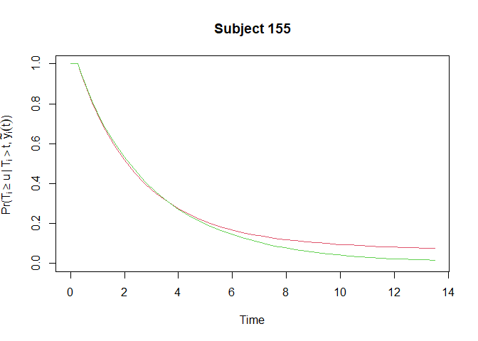
Step 3
Using the first measurement of Patient 155, and the fitted joint model
calculate the conditional survival probabilities via survfitJM()
sfit = survfitJM(joint.fit, newdata = dataP155[1:2,])
plot(sfit)
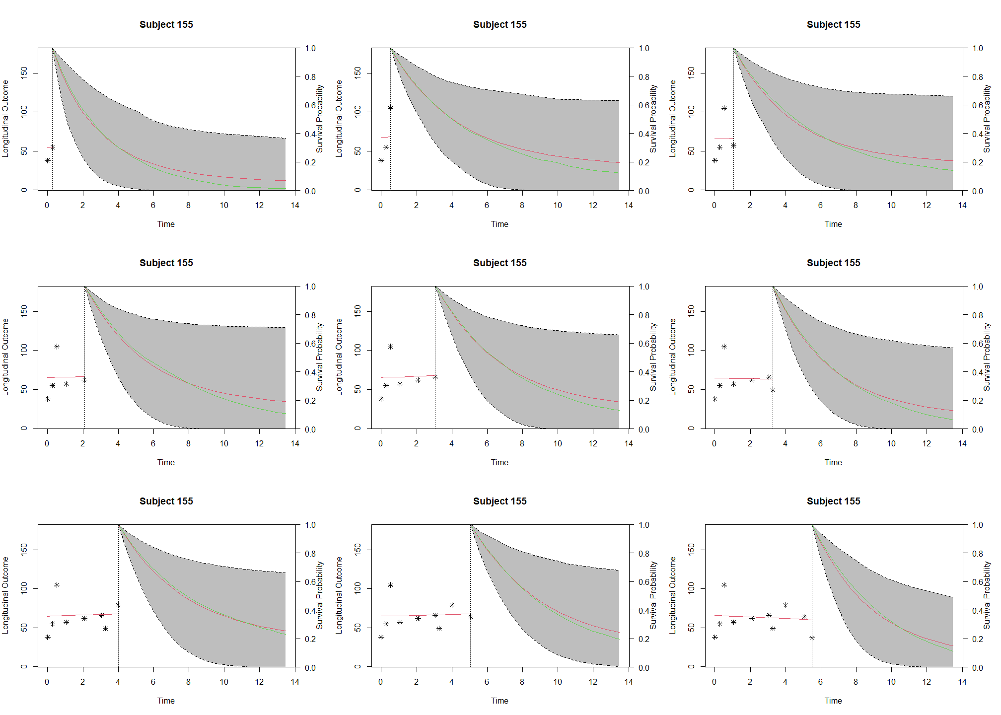
Step 4
n155 = nrow(dataP155) # 10
# par(mfrow=c(as.integer(n155/2),2)) ## error: margins too large
for (i in 2:n155) {
  sfit = survfitJM(joint.fit, newdata = dataP155[1:i,])
  plot(sfit, include.y = TRUE, conf.int = TRUE, fill.area = TRUE)
}