Gaussian Processes for Regression
Posted on
This note is for Chapter 4 of Rasmussen, C. E., & Williams, C. K. I. (2006). Gaussian processes for machine learning. MIT Press.
Dataset $\cD$ of $n$ observations, $\cD=\{(\x_i,y_i)\mid i=1,\ldots,n\}$
move from the finite training data $\cD$ to a function $f$ that makes predictions for all possible input values.
Two common approaches:
- restrict the class of functions, such as only considering linear functions of the input
- give a prior probability to every possible function, where higher probabilities are given to functions that we consider to be more likely, for example because they are smoother than other functions.
A Gaussian process is a generalization of the Gaussian probability distribution.
Several ways to interpret Gaussian process (GP) regression models.
- function-space view: think of a GP as defining a distribution over functions
- weight-space view:
Weight-space view
The Standard Linear Model
\[f(x) = x^Tw, \qquad y=f(x) + \varepsilon, \qquad \varepsilon \sim N(0, \sigma_n^2)\]Put a zero mean Gaussian prior with covariance matrix $\Sigma_p$ on the weights
\[w\sim N(0, \Sigma_p)\]we can obtain
\[p(w\mid X, y) \sim N(\bar w, A^{-1})\]where the mean is also its mode, which is also called the maximum a posterior (MAP) estimate of $w$.
In a non-Bayesian setting, the negative log prior is sometimes thought of as a penalty term, and the MAP point is known as the penalized maximum likelihood estimate of the weights.
To make predictions for a test case, we average over all possible parameter values, weighted by their posterior probability. Thus the predictive distribution for $f_\star$ at $x_\star$ is given by averaging the output of all possible linear models w.r.t. the Gaussian posterior,
\[p(f_\star\mid x_\star,X,y) = \int p(f_\star\mid x_\star,w)p(w\mid X, y)dw\]Projections of Inputs into Feature Space
Introduce the function $\phi(x)$ which maps a D-dimensional input vector $x$ into an $N$ dimensional feature space.
\[f(x) = \phi(x)^Tw\]Define $k(x,x’)=\phi(x)’\Sigma_p\phi(x’)$ as a covariance function or kernel.
kernel trick: if an algorithm is defined solely in terms of inner products in input space then it can be lifted into feature space by replacing occurrences of those inner products by $k(x,x’)$.
Function-space View
A Gaussian process is a collection of random variables, any finite number of which have a joint Gaussian distribution.
A GP is completely specified by its mean function and covariance function,
\[f(x) \sim GP(m(x), k(x, x'))\]marginalization property: if the GP specifies $(y_1,y_2)\sim N(\mu,\Sigma)$, then it must also specify $y_1\sim N(\mu_1,\Sigma_{11})$
squared exponential (SE) covariance function:
\[\cov(f(x_p), f(x_q)) = k(x_p,x_q) = \exp(-\frac 12\vert x_p-x_q\vert^2)\]The specification of the covariance function implies a distribution over functions. We can draw samples from the distribution of functions evaluated at any number of points.
Varying the Hyperparameters
The SE covariance function in one dimension has the following form
\[k_y(x_p, x_q) = \sigma_f^2 \exp\left(-\frac{1}{2\ell^2}(x_p-x_q)^2\right) + \sigma^2_n\delta_{pq}\]Other kernel functions,
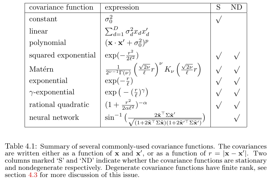
The Matérn Class of Covariance Functions
- $\nv \rightarrow\infty$, it becomes the SE kernel
- it becomes simple when $\nv$ is half-integer: $\nv = p+1/2$. In this case, the covariance function is a product of an exponential and a polynomial of order $p$
- for $\nv \ge 7/2$, in the absence of explicit prior knowledge about the existence of higher order derivatives, it is probably very hard from finite noisy training examples to distinguish between values of $\nv \ge 7/2$ (or even to distinguish between finite values of $\nv$ and $\nv\rightarrow\infty$)
Rational Quadratic Covariance Function
It can be seen as a scale mixture (an infinite sum) of squared exponential (SE) covariance functions with different characteristic length-scales
if $\alpha\rightarrow\infty$, the limit of the RQ covariance is the SE covariance function